This article is originally from the book "Computer Vision with PyTorch"
In the previous chapter, we learned about R-CNN and Fast R-CNN techniques, which leveraged region proposals to generate predictions of the locations of objects in an image along with the classes corresponding to objects in the image. Furthermore, we learned about the bottleneck of the speed of inference, which happens because of having two different models-one for region proposal generation and another for object detection. In this chapter, we will learn about different modern techniques, such as Faster R-CNN, YOLO, and Single-Shot Detector (SSD), that overcomes slow inference time by employing a single model to make predictions for both the class of objects and the bounding box in a single shot. We will start by learning about anchor boxes and then proceed to learn about how each of the techniques works and how to implement them to detect objects in an image.
Components of modern object detection algorithms
The drawback of the R-CNN and Fast R-CNN techniques is that they have two disjointed networks-one to identify the regions that likely contain an object and the other to make corrections to the bounding box where an object is identified. Furthermore, both the models require as many forward propagations as there are region proposals. Modern object detection algorithms focus heavily on training a single neural network and have the capability to detect all objects in one forward pass. In the subsequent sections, we will learn about the various components of a typical modern object detection algorithm:
- Anchor Boxes
- Region Proposal Network (RPN)
- Region of Interest Pooling (RoI)
Anchor boxes
So far, we have region proposals coming from the selective search method. Anchor boxes come in as handy replacement for selective search-we will learn how they replace selective search-based region proposals in this section.
Typically, a majority of objects have a similar shape-for example, in a majority of cases, a bounding box corresponding to an image of a person will have a greater height than width, and a bounding box corresponding to the image of a truck will have a greater width than height. Thus, we will have a decent idea of the height and width of the objects present in an image even before training the model (by inspecting the ground truths of bounding boxes corresponding to objects of various classes).
Furthermore, in some images, the objects of interest might be scaled-resulting in a much smaller or much greater height and width than average-while still maintaining the aspect ratio (that is, ).
Once we have a decent idea of the aspect ratio and the height and width of objects (which can be obtained from ground truth values in the dataset) present in our images, we define the anchor boxes with heights and widths representing the majority of objects' bounding boxes within our dataset.
Typically, this is obtained by employing K-means clustering on top of the ground truth bounding boxes of objects present in images.
Now that we understand how anchor boxes' heights and widths are obtained, we will learn about how to leverage them in the process:
- Slide each anchor box over an image from top left to bottom right
- The anchor box that has a high intersection over union (IoU) with the object will have a label that it contains an object, and the others will be labeled 0.
- We can modify the threshold of the IoU by mentioning that if the IoU is greater than a certain threshold, the object class is 1; if it is less than another threshold, the object class is 0, and it is unknown otherwise. Once we obtain the ground truths as defined here, we can build a model that can predict the location of an object and also the offset corresponding to the anchor box to match it with ground truth. Let's understand how anchor boxes are represented in the following image:
 In the preceding image, we have two anchor boxes, one that has a greater height than width and the other with a greater width than height, to correspond to the objects (classes) in the image-a person and a car.
- We can modify the threshold of the IoU by mentioning that if the IoU is greater than a certain threshold, the object class is 1; if it is less than another threshold, the object class is 0, and it is unknown otherwise. Once we obtain the ground truths as defined here, we can build a model that can predict the location of an object and also the offset corresponding to the anchor box to match it with ground truth. Let's understand how anchor boxes are represented in the following image:
We slide the two anchor boxes over the image and note the locations where the IoU of the anchor box with the ground truth is the highest and denote that this particular location contains an object while the rest of the locations do not contain an object.
In addition to the preceding two anchor boxes, we would also create anchor boxes with varying scales so that we accommodate the different scales at which an object can be presented within an image. An example of how the different scales of anchor boxes look follows:  Note that all the anchor boxes have the same center but different aspect ratios or scales.
Now that we understand anchor boxes, in the next section, we will learn about the RPN, which leverages anchor boxes to come up with predictions of regions that are likely to contain an object.
Region Proposal Network
Imagine a scenario where we have a 224x224x3 image. Furthermore, let's say that the anchor box is of shape 8x8 for this example. If we have a stride of 8 pixels, we are fetching 224/8 = 28 crops of a picture for every row-essentially crops from a picture. We then take each of these crops and pass through a Region Proposal Network (RPN) model that indicates whether the crop contains an image. Essentially, an RPN suggests the likelihood of a crop containing an object.
Let's compare the output of selectivesearch and the output of an RPN.
selectivesearch gives a region candidates based on a set of computations on top of pixel values. However, an RPN generates region candidates based on the anchor boxes and strides with which anchor boxes are slid over the image. Once we obtain the region candidates using either of these two methods, we identify the candidates that are most likely to contain an object.
While region proposal generation based on selectivesearch is done outside of the neural network, we can build an RPN that is part of the object detection network. Using an RPN, we are now in a position where we don't have to perform unnecessary computations to calculate region proposals outside of the network. This way, we have a single model to identify regions, identify classes of objects in image, and identify their corresponding bounding box locations.
Next, we will learn how an RPN identifies whether a region candidate (a crop obtained after sliding an anchor box) contains an object or not. In our training data, we would have the ground truth correspond to objects. We now take each region candidate and compare with the ground truth bounding boxes of objects in an image to identify whether the IoU between a region candidate and a ground truth bounding box is greater than a certain threshold (say, 0.5). If the IoU is greater than a certain threshold, the region candidate contains an object, and if the IoU is less than a threshold (say 0.1), the region candidate does not contain an object and all the candidates that have an IoU between the two thresholds (0.1-0.5) are ignored while training.
Once we train a model to predict if the region candidate contains an object, we then perform non-max suppression, as multiple overlapping regions can contain an object.
In summary, an RPN trains a model to enable it to identify region proposals with a high likelihood of containing an object by performing the following steps:
- Slide anchor boxes of different aspect ratios and sizes across the image to fetch crops of an image.
- Calculate the IoU between the ground truth bounding boxes of objects in the image and the crops obtained in the previous step.
- Prepare the training dataset in such a way that crops with an IoU greater than a threshold contain an object and crops with an IoU less than a threshold do not contain an object.
- Train the model to identify the regions that contain an object.
- Perform non-max suppression to identify the region candidate that has the highest probability of containing an object and eliminate other region candidates that have a high overlap with it.
Classification and regression
So far, we have learned about the following steps in order to identify objects and perform offsets to bounding boxes:
- Identify the regions that contain objects.
- Ensure that all the feature maps of regions, irrespective of the regions' shape, are exactly the same using Region of Interest (RoI) pooling.
Two issues with these steps are as follows:
- The region proposals do not correspond tightly over the object (IoU>0.5 is the threshold we had in the RPN).
- We identified whether the region contains an object or not, but not the class of the object located in the region.
We address these two issues in this section, where we take the uniformly shape feature map obtained previously and pass it through a network. We expect the network to predict the class of the object contained within the region and also the offsets corresponding to the region to ensure that the bounding box is as tight as possible around the object in the image.
Let's understand this through the following diagram: 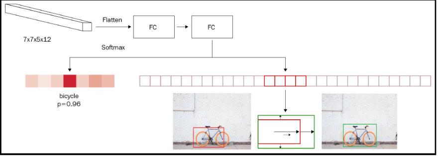 In the preceding diagram, we are taking the output of RoI pooling as input (the 7x7x5x12 shape), flattening it, and connecting to a dense layer before predicting two aspects:
- Class of object in the region
- Amount of offset to be done on the predicted bounding boxes of the region to maximize the IoU with the ground truth
Hence, if there are 20 classes in the data, the output of the neural network contains a total of 25 outputs-21 classes (including the background class) and the 4 offsets to be applied to the height, width, and two center coordinates of the bounding box.
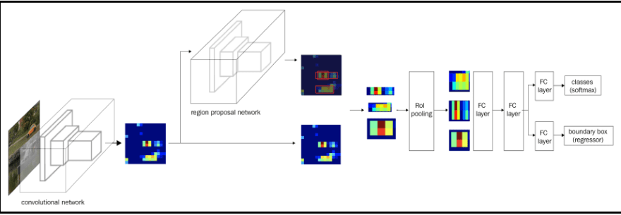
Now that we have learned the different components of an object detection pipeline, let's summarize it with the following diagram:
Working details of YOLO
You Only Look Once (YOLO) and its variants are one of the prominent object detection algorithms. In this section, we will understand at a high level how YOLO works and the potential limitations of R-CNN-based object detection frameworks that YOLO overcomes.
First, let's learn about the possible limitations of R-CNN-based detection algorithms. In Faster R-CNN, we slide over the image using anchor boxes and identify the regions that are likely to contain an object, and then we make the bounding box corrections. However, in the fully connected layer, where only the detected region's RoI pooling output is passed as input, in the case of regions that do not fully encompass the object (where the object is beyond the boundaries of the bounding box of region proposal), the network has to guess the real boundaries of object, as it has not seen the full image (but has seen only the region proposal).
YOLO comes in handy in such scenarios, as it looks at the whole image while predicting the bounding box corresponding to an image.
Furthermore, Faster R-CNN is still slow, as we have two networks: the RPN and the final network that predicts classes and bounding boxes around objects.
Here, we will understand how YOLO overcomes the limitations of Faster R-CNN, both by looking at the whole image at once as well as by having a single network to make predictions.
We will look at how data is prepared for YOLO through the following example:
- Create ground truth to train a model for a given image:
- Let's consider an image with the given ground truth of bounding boxes in red:

- Divide the image into NxN grid cells-for now, let's say N=3:

- Identify those grid cells that contain the center of at least one ground truth bounding box. In our case, they are cells b1 and b3 of our 3x3 grid image.
- The cell(s) where the middle point of ground truth bounding box falls is/are responsible for predicting the bounding box of the object. Let's create the ground truth corresponding to each cell.
- The output ground truth corresponding to each cell is as follows:
 Here, pc (the objectness score) is the probability of the cell containing an object.
- Let's consider an image with the given ground truth of bounding boxes in red:
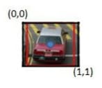
Let's understand how to calculate bx, by, bw and bh.
First, we consider the grid cell (let's consider the b1 grid cell) as our universe, and normalize it to a scale between 0 and 1, as follows:
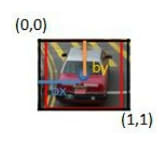
bx and by are the locations of the mid-point of the ground truth bounding with respect to the image (of the grid cell), as defined previously. In our case, bx = 0.5, as the mid-point of the ground truth is at a distance of 0.5 unit from the origin. Similarly, by = 0.5.
So far, we have calculated offsets from the grid cell center to the ground truth center corresponding to the object in the image. Now, let's understand how bw and bh are calculated.
bw is the ratio of the width of the bounding box with respect to the width of the grid cell.
bh is the ratio of the height of the bounding box with respect to the height of the grid cell.
Next, we will predict the class corresponding to the grid cell. If we have three classes, we will predict the probability of the cell containing an object among any of the three classes. Note that we do not need a background class here, as pc corresponds to whether the grid cell contains an object.
Now that we understand how to represent the output layer of each cell, let's understand how we construct the output of our 3x3 grid cells.
Let's consider the output of the grid cell a3:

The output of cell a3 is as shown in the preceding screenshot. As the grid cell does not contain an object, the first output (pc-objectness score) is 0 and the remaining values do not matter as the cell do not contain the center of any ground truth bounding box of an object.Let's consider the output corresponding to grid cell b1:

The preceding output is the way it is because the grid cell contains an object with the bx, by, bw, and bh values that were obtained in the same way as we went through earlier (in the bullet point before last), and finally the class being car resulting in c2 being 1 while c1 and c3 are 0.
Note that for each cell, we are able to fetch 8 outputs. Hence, for 3x3 grid of cells, we fetch 3x3x8 outputs.
Define a model where the input is an image and the output is 3x3x8 with the ground truth being as defined in the previous step.

Define the ground truth by considering the anchor boxes.
So far, we have been building for a scenario where the expectation is that there is only one object within a grid cell. However, in reality, there can be scenarios where there are multiple objects within the same grid cell. This would result in creating ground truths that are incorrect. Let's understand this phenomenon through the following example image:

In the preceding example, the mid-point of the ground truth bounding boxes for both the car and the person fall in the same cell-cell b1.
One way to avoid such a scenario is by having a grid that has more rows and columns-for example, a 19x19 grid. However, there can be still a scenario where an increase in the number of grid cells does not help. Anchor boxes come in handy in such a scenario. Let's say we have two anchor boxes-one that has a greater height than width (corresponding to the person) and another that has a greater width than height (corresponding to the car):

Typically the anchor boxes would have the grid cell center as their centers. The output for each cell in a scenario where we have two anchor boxes is represented as a concatenation of the output expected of the two anchor boxes:

Here, bx, by, bw and bh represent the offset from the anchor box (which is the universe in this scenario as seen in the image instead of the grid cell).
From the preceding screenshot, we see we have an output that is 3x3x16, as we have two anchors. The expected output is of the shape NxNx(num_classes+1)x(num_anchor_boxes), where *NxN is the number of cells in the grid, num_classes is the number of classes in the dataset, and num_anchor_boxes is the number of anchor boxes.
- Now we define the loss function to train the model.
When calculating the loss associated with the model, we need to ensure that we do not calculate the regression loss and classification loss when the objectness score is less than a certain threshold (this corresponds to the cells that do not contain an object).
Next, if the cell contains an object, we need to ensure that the classification across different classes is as accurate as possible.
Finally, if the cell contains an object, the bounding box offsets should be as close to expected as possible. However, since the offsets of width and height can be much higher when compared to the offset of the center (as offsets of the center range between 0 and 1, while the offsets of width and height need not), we give a lower weightage to offsets of width and height by fetching a square root value.
Calculate the loss of localization and classification as follows:


Here, we observe the following:
- lambda_coordinate is the weightage associate with regression loss.
- object_ij represents whether the cell contains an object.
- hat_p_i(c) corresponds to the predicted class probability, and C_ij represents the objectness score.
The overall loss is a sum of classification and regression loss values.
Working details of SSD
So far, we have seen a scenario where we made predictions after gradually convolving and pooling the output from the previous layer. However, we know that different layers have different receptive fields to the original image. For example, the initial layers have a smaller receptive field when compared to the final layers, which have a larger receptive field. Here, we will learn how SSD leverages this phenomenon to come up with a prediction of bounding boxes for images.
The workings behind how SSD helps overcome the issue of detecting objects with different scales is as follows:
- We leverage the pre-trained VGG network and extend it with a few additional layers until we obtain a 1x1 block.
- Instead of leveraging only the final layer for bounding box and class predictions, we will leverage all of the last few layers to make class and bounding box predictions.
- In place of anchor boxes, we will come up with default boxes that have a specific set of scales and aspect ratios.
- Each of the default boxes should predict the object and bounding box offset just like how anchor boxes are expected to predict classes and offsets in YOLO.
Now that we understand the main ways in which SSD differs from YOLO (which is that default boxes in SSD replace anchor boxes in YOLO and multiple layers are connected to the final layer in SSD, instead of gradual convolution pooling in YOLO), let's learn about the following:
- The network architecture of SSD
- How to leverage different layers for bounding box and class predictions
- How to assign scale and aspect ratios for default boxes in different layers

Top comments (0)