
In this article, I'd like to introduce the basic concepts required to implement a simple neural network from scratch. Even though this neural network is rather primitive by modern standards, it can still do something that's actually quite useful and impressive: It can be trained to accurately recognize handwritten digits between 0 and 9!
I recently went over a few different tutorials on the subject. While those tutorials were great, at the end of it I thought there was room to clarify some things a bit further. In addition to this primer, you may want to check out the following free resources as well:
- Neural Networks, a youtube video series by 3Blue1Brown (Grant Sanderson)
- Chapters one and two of Neural Networks and Deep Learning, by Michael Nielsen
Neural Network Structure
The structure of our neural network is quite simple. The basic unit of the network is the neuron. Each neuron can have inputs from any number of neurons feeding into it. A neuron produces a single output value, which is called the activation for that neuron. This activation value can in turn be sent as input to any number of other neurons.
The neurons are organized into layers. Each neuron in a given layer receives inputs from all of the neurons in the previous layer. The activation of a given neuron is also sent to all of the neurons in the next layer. The first layer is called the input layer. The last layer is called the output layer. Any layers in between are called hidden layers, because they only affect the ultimate output of the network indirectly. We can think of this as an assembly line: The raw materials go into the input layer and the final product comes out the other end from the output layer. All of the intermediate steps involved in building the end product occur in the hidden layers. Below is a simple diagram showing the basic structure of a neural network:
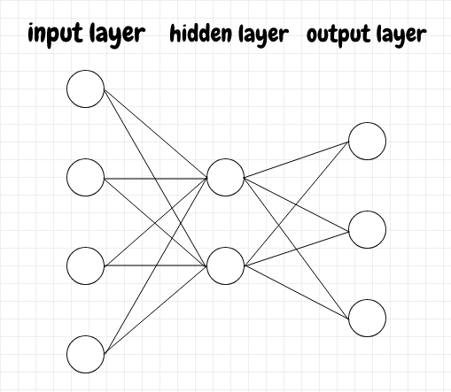
The network shown above has a single hidden layer, but there are often multiple hidden layers.
The edge connecting two neurons has two values associated with it. There's the activation of the sending neuron as well as a weight assigned to that activation by the receiving neuron. The higher the weight, the more significantly the incoming activation will affect the receiving neuron's activation. A given neuron may receive inputs from many neurons, and each will have its own weight. Each neuron also has an additional value called the bias. The bias is a measure of how intrinsically active a neuron is. A high positive bias means that the neuron will tend to have a higher activation regardless of what inputs it receives. A high negative bias will act as a brake, significantly dampening the activation of the neuron.
For this example, we will restrict the activation of a given neuron to a value between 0 and 1. To accomplish this, we'll use the sigmoid function. This function takes any positive or negative number as input and squashes it into a range between 0 and 1. Below is the diagram and formula for the sigmoid function:

Sigmoids were used early on in the history of neural networks, but they are not used very much any more. These days, something like a ReLU function is more common.
Below we have the simplest case of a single neuron in layer L feeding into a neuron in the next layer, L+1. To calculate the activation for the neuron in layer L+1, first we multiply the weight for that edge by the activation from the sending neuron, then we add the bias. This becomes a raw activation value that we will call z in this article. Lastly, we apply the sigmoid function to z to obtain the actual activation, a, for the neuron in the next layer, L+1.

Input and Output
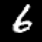
Grant Sanderson calls recognizing the mnist numbers the hello world of neural networks. The input images come from the mnist database. Each mnist image is a 28 x 28 grid of pixels. Each pixel is a decimal number between 0 and 1 and represents a greyscale value. The image below of a 6 is an example of what an mnist image looks like:
To supply these values as inputs into the network, we simply line up all of the pixels into a single column, and assign the greyscale value for each pixel to a corresponding input neuron. That means we need 28 x 28, or 784 input neurons.
To clarify, see the diagram below of the number 2 represented as a simple 6x6 grid. The real mnist images have greyscale values, but in this example the cells are either black or white (0 or 1). To generate an input layer, we assign the first row of pixels as input neurons, then the next row below that, and so on. The end result is that our input is represented by 36 neurons:

Our network for recognizing handwritten digits uses 10 output neurons, each with values between 0 and 1. We want the output neuron corresponding to the correct digit to light up with a value close to 1 and for all of the other neurons to be as close to 0 as possible. If our image represents the digit 4, that means we want our output neurons to indicate something close to [0, 0, 0, 0, 1, 0, 0, 0, 0, 0].
Why do we use 10 output neurons? After all, we could compress the output. For example, in binary we could encode the digits from 0 to 10 with 4 neurons. This would work, but it seems as though simplifying the output, so that each output neuron has only a single meaning, makes it easier for the network to learn. Conceptually, it means that when we tug to increase or decrease the activation for an output neuron, there is only one meaning to it.
The diagram below shows an overview of the neural network that's actually used in Michael Nielsen's book to recognize the mnist images:

image credit: Michael A. Nielsen, "Neural Networks and Deep Learning", Determination Press, 2015
Gradient Descent
The key idea behind neural networks is gradient descent. What is gradient descent? Let's say you're taking a walk in a lush green region of hills and meadows. Suppose you're at the top of a hill and you want to get down into the valley. However, you've been blindfolded, so you can't see where you're going. How can you get to the bottom? A simple approach is simply to slowly spin around in place, and feel with your feet to find the steepest part of the hill at your current location, then to take a small step downward along that slope. From there you can again feel around for what seems to be the steepest downward slope, and take another small step in that direction, and so on. Eventually you'll reach a flat region where the slope has tapered off. This method doesn't guarantee that you will find the best path into the valley, but it does make sure that each step is the best move locally relative to where you are at that point in time.
In a nutshell, this is the gradient descent approach used by neural networks! It's really that simple. Every problem that neural networks solve, whether it's image and speech recognition, or playing the game of go, or predicting the stock market, is ultimately represented as some function with a very large number of variables. We can intuitively think of it as a huge (multi-dimensional) landscape. The job of the neural network becomes to iterate over a large amount of data in order to tune those variables so that it can move downward along the slope of this very complicated function.
Partial Derivatives and Gradients
Let's explore this idea of gradient descent with some simple math. Let's say we have a function f over a single variable x. As we adjust the variable x, the value of the function, f(x), changes accordingly.
If we're at some point x right now, how can we take a step downward along this function? We can calculate the local slope of the function by taking the derivative of f with respect to x. If the derivative, ∂f(x)/x, is positive, that means the function is trending upward. If the derivative is negative, it means the function is trending downward. We can therefore calculate our step in the downward direction with the following pseudo code, where step_size is a small increment value that we've chosen ahead of time:
step = ∂f(x)/x * step_size
x = x - step
- If
∂f(x)/xis positive, thenstepwill also be positive. Therefore subtractingstepfromxwill makexsmaller. A smallerxwill cause f(x) to be smaller as well. In other words, we're moving downhill. - If the derivative is negative, then
stepwill also be negative. Subtracting a negative value is the same as adding a positive value, so in this casexwill increase. Since the slope is negative, increasingxwill cause us to go downhill.
Therefore x = x - step will help us to go downhill regardless of whether the slope is positive or negative. If the slope becomes 0, then we've reached a flat region. This is called a local minimum of the function.
The notation ∂f(x)/x tells us that if we make a small change to x, it will have have a certain effect on f(x). If this value is very high (either in the positive or negative direction), that means the slope is steep. A small step in the x direction will cause us to take a big step up or down the function. If the value is close to 0, it means the slope is relatively flat, so a step in the x direction won't change our elevation very much.
Choosing a good value for
step_sizedepends on the problem at hand. Making it too small will tend to slow down the network's learning, but making it too big could potentially mean that a single step takes us to a higher point in the function, instead of going downward, which is also undesirable. Because of its effect on learning,step_sizeis often called the learning rate in neural network terminology. It's a hyperparameter. The term hyperparameter sounds complicated, but it simply means that learning rate is a parameter that has to be manually tuned rather than being refined by the network itself as it learns. Any parameter that we select for our neural network that doesn't then get fine-tuned by the network's learning process is called a hyperparameter. We can think of the hyperparameters as dials and knobs that we can tweak prior to starting the learning process. These are values that will affect the learning process of the network, but the feedback loop of training the network won't alter these parameters. They stay the same unless we manually adjust them.
We've looked at a function of a single variable x. Such functions can be viewed as graphs in 2 dimensions, with one axis for x and one for f(x), like in the diagram below:

If we increase the function to 2 variables, f(x,y), then we need one axis for each of x and y to represent the inputs, and the function can therefore be viewed as a graph in 3 dimensions. The slope of this function also becomes a vector in 3 dimensions. We can decompose this vector into two component vectors, the slope along the x axis and the slope along the y axis. These two values, ∂f(x,y)/x, and ∂f(x,y)/y, are called the partial derivatives of the function with respect x and y. In other words, ∂f(x,y)/x tells us how much f(x,y) will change if we make a small adjustment to x and leave y unchanged. Conversely, ∂f(x,y)/y tells us how f(x,y) will change if we make a small adjustment to y while leaving x the same. The list of the partial derivatives, [∂f(x,y)/x, ∂f(x,y)/y], is called the gradient of the function. It defines the slope of the function in the direction of steepest descent, in the sense that adding these partial derivative vectors together produces the overall gradient vector.
This idea also applies to functions with a larger number of parameters, f(x,y,z,...). In fact, that's precisely how neural networks operate. We can't directly visualize such functions, but we can use the same mathematical tools to get the gradient. To move downward along such a gradient with our small steps, we apply the same trick of subtracting from each variable the partial derivative with respect to that variable times some small step size. The adjusted values for each axis will result in a smaller f(x,y,z...). In other words, this moves the function downward along the steepest path of descent relative to its current location. When we look at the math that accomplishes this later on, I think it's helpful to keep in mind that, at a high level, this is all that's happening.
Activation
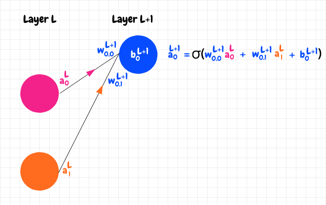
Let's calculate the outputs for our network. We've already seen how to calculate the activation for a neuron that has only a single input. When a neuron has multiple neurons feeding into it, we add up the weighted activations from the incoming neurons first, then we add the bias, and finally we apply our sigmoid function. In other words, all of the incoming activity affects how active our neuron becomes. Let's say we have a neuron in layer L+1 with 2 neurons feeding into it, as in the diagram below:
The superscripts L and L+1 are not exponents. They just signify which layer of the network the value belongs to. Please do keep in mind that (almost) any time you see superscripts in this article, they do not denote an exponent! The only exceptions are the sigmoid function and its derivative, and the 2 used as the exponent for the quadratic cost function.
We can see that we add the weighted activations from the pink and orange neurons and add the bias of the blue neuron to produce the raw activation for the blue neuron, z: z = w0,0L+1a0L + w0,1L+1a1L + b0L+1. Then we apply the sigmoid function to obtain the activation: a = σ(z).
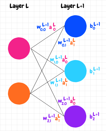
It turns out that we can express this calculation neatly using matrices. Let's index the neurons in layer L+1 with j, and the neurons in the previous layer L with k. J will denote the total number of neurons in layer L+1 and K will denote the total number of neurons in layer L.
This ordering of j and k may look backwards but we'll see why we use this indexing scheme in a moment.
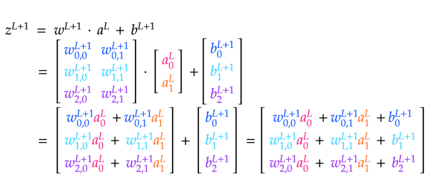
Let's consider a simple neural network with two layers. The first layer, L, has 2 neurons and the second layer, L+1, has 3 neurons:
We want the activations for layer L+1 to be a 3x1 matrix, that is, a matrix with 3 rows in a single column. The value in each row will represent the activation for the corresponding neuron in that layer. To get our results into the appropriate form, we can define the needed matrices as follows:
First, we define a matrix wL+1 for the weights coming into layer L+1 as a JxK matrix. The first row of this matrix will contain each of the weights coming into the first neuron in layer L+1; the second row will have each of the weights coming into the second neuron in layer L+1, and so on.
Next, we group the activations in layer L into a Kx1, single-column matrix, aL. The first row has the activation coming from the first neuron in layer L; the second row has the activation coming from the second neuron in layer L, and so on.
Lastly we place the biases for the neurons in layer L+1 into a Jx1, single-column matrix, bL+1. The first row has the bias for the first neuron in layer L+1; the second row has the bias for the second neuron in layer L+1, etc.
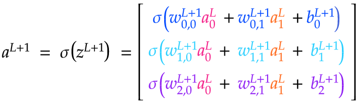
We can see that taking the dot product of wL+1 ⋅ aL produces a Jx1 matrix. We can add that matrix to bL+1, also Jx1, which produces a Jx1 matrix zL+1 that has all of the raw activation values for layer L+1. Finally we can just pass each of the values in zL+1 to σ to obtain a matrix aL+1 of the activations for layer L+1.
We can see that we need to arrange the weights matrix w for a given layer L+1 such that each row corresponds to the edges coming into a given neuron in layer L+1. This makes intuitive sense, since the activation for a neuron in L+1 depends on all of the inputs coming in from the previous layer. That's why we use j to index the neurons in the next layer and k to index the neurons in the previous layer, because we want the weights matrix to be a JxK matrix. That way, the dot product will work out to produce the correct shape for the z and a matrices. If we did the indexing the other way around, our weights matrix would be a KxJ matrix. That would be fine too, since the meaning of the rows and columns wouldn't change, just the nomenclature. Below are the matrix calculations needed to compute zL+1 and aL+1:
Calculating the dot product of two matrices is fairly simple. The two matrices must have the form I x J and J x K such that the result becomes an I x K matrix. In other words, the number of columns for the matrix on the left must match the number of rows for the matrix on the right. The dot product becomes a matrix with the same number of rows as the matrix on the left and the same number of columns as the matrix on the right.
Cost Function
In order for the network to learn, we need to provide feedback about whether the current network performed well for a given training input. This is done by using a cost function. The cost function compares the network's actual output against the correct value. We may have multiple neurons in the output layer. In that case we need to compare the correct values for each of the output neurons against each actual output. For this example, we'll use a simple function called the quadratic cost function:
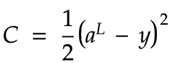
As far as I can tell, the extra division by 2 is mostly there to cancel the factor of 2 that we obtain when we take the derivative of this function. In any case, this constant factor should not significantly affect how the network learns.
If our network only has a single output neuron, then the cost can be calculated by subtracting the correct value from the output value, and then squaring that result. If we have multiple output neurons, like the 10 neurons in our mnist number recognition network, then we can treat aL, the actual output, and y, the correct values, as single column matrices. In that case, we subtract these two matrices. This amounts to performing the same subtraction for each row of the resulting matrix. We subtract the expected value for each given neuron from its corresponding actual output, then square the result.
For a given value of a and y, if we map these as points on a line, we can see that a - y is the distance between the two points, so the cost function is the square of this distance. There are other cost functions that are used in machine learning as well.
Backpropagation
We want to adjust the weights and the biases in our network such that, over time, the training data will yield a lower and lower cost. To do so, we'll need to figure out the slope of the cost function with respect to these weights and biases. Then we can use gradient descent to move down this slope in small steps for each feedback loop of the network.
Let's consider a minimalistic scenario where we have a single output neuron with a single neuron feeding into it from a hidden layer. It turns out that the equations we derive for this trivial case are easy to adapt to the more general case of multiple neurons per layer.
In the diagram below, we can see that the cost, C, for the output depends directly on the activation aL and on the expected value for that input, y. In turn, aL depends on the raw activation, zL. Lastly, zL depends on 3 variables: The bias, bL, the weight, wL, and the incoming activation, aL-1:

We will use this information to figure out the derivative of the cost function with respect to the weight and bias. We will also determine the derivative of the cost with respect to the activation of the neuron in the previous layer. You may wonder why we'd need to determine the cost function relative to the activation in the previous layer. After all, we can't directly adjust it. That is indeed true, we can't modify a neuron's activation directly. However, we will be able to use the gradient with respect to the activation in the previous layer to calculate the needed changes to the weights and biases for that previous layer, and so on, moving backward through the network. This is why we call this step of adjusting all of the weights and biases backpropagation.
Let's first calculate the derivative of the cost function with respect to the activation of the output neuron. This is quite simple. The derivative is just a linear function:

Since aL depends on zL, let's also figure out the slope of a with respect to z:
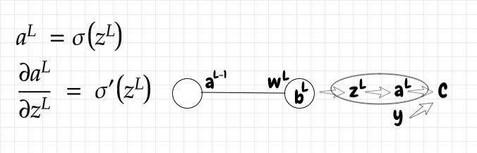
The derivative of the sigmoid function is:

zL depends on the incoming activation from the previous layer, aL-1, the weight for that activation, wL, and the current bias, bL. Let's compute the partial derivatives of z with respect to each of these inputs:

Now that we have all of the partial derivatives we need, we can use the chain rule to compute the 3 equations we'll need to do backpropagation for our network: The partial derivative of the cost function with respect to the weight, the bias, and the previous layer's activation:

The idea is that we can calculate ∂C/∂aL-1 using the values of wL and ∂C/dbL. Once we have ∂C/∂aL-1, we can use it to calculate ∂C/dbL-1 and ∂C/dwL-1. From there we just keep repeating the same steps backward through the layers of our network until we reach the input layer, hence the term backpropagation.
Example Calculation
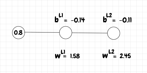
Let's compute a single learning iteration for a small network with a single input neuron, one middle neuron, and a single output neuron. We'll set the input to 0.8. The expected output, y, is 1 for this input. The weights and biases are in the diagram below:
First we need to calculate the raw activations z as well as the activations a for the network. We use the following (python) functions for z, a, and sigmoid:
import numpy as np

def sigmoid(z):
    return 1.0/(1.0+np.exp(-z))

def z(w, a, b):
    return w * a + b

def a(z):
    return sigmoid(z)
For layer L1, we can calculate the value of z and a as follows:
>>> a_l0 = 0.8
>>> w_l1 = 1.58
>>> b_l1 = -0.14
>>> z_l1 = z(w_l1, a_l0, b_l1)
>>> a_l1 = sigmoid(z_l1)
>>> z_l1
1.124
>>> a_l1
0.7547299213576082
Now that we have the activation for layer L1, we can use it to calculate z and a for layer L2:
>>> b_l2 = -0.11
>>> w_l2 = 2.45
>>> z_l2 = z(w_l2, a_l1, b_l2)
>>> a_l2 = sigmoid(z_l2)
>>> z_l2
1.73908830732614
>>> a_l2
0.850571226530534
Great, now we've got our activation for L2. We now need to calculate the slope of the cost function with respect to three variables, the bias, the weight, and the activation from the previous layer. The equations for the partial derivatives, as well as the derivative of the sigmoid function, sigmoid_prime are below:
def sigmoid_prime(z):
    return sigmoid(z)*(1-sigmoid(z))

def dc_db(z, dc_da):
    return sigmoid_prime(z) * dc_da

def dc_dw(a_prev, dc_db):
    return a_prev * dc_db

def dc_da_prev(w, dc_db):
    return w * dc_db
We calculate these partial derivatives below:
>>> dc_da_l2 = a_l2-1
>>> dc_db_l2 = dc_db(z_l2, dc_da_l2)
>>> dc_dw_l2 = dc_dw(a_l1, dc_db_l2)
>>> dc_da_l1 = dc_da_prev(w_l2, dc_db_l2)
>>> dc_db_l2
-0.018992369482903983
>>> dc_dw_l2
-0.014334109526226761
>>> dc_da_l1
-0.04653130523311476
Now that we have the slope of the cost function with respect to the bias b_l2 and the weight w_l2, we can update those biases and weights:
>>> step_size = 0.1
>>> updated_b_l2 = b_l2 - dc_db_l2 * step_size
>>> updated_w_l2 = w_l2 - dc_dw_l2 * step_size
>>> updated_b_l2
-0.1081007630517096
>>> updated_w_l2
2.451433410952623
Having adjusted the weight and bias for the L2 layer, we can do the same thing for the L1 layer. We've calculated dc_da_l1, which is the slope of the cost function with respect to the activation coming from the previous layer. To obtain the gradient for the bias and weight for the L1 layer, we just continue using the chain rule as before. In the L2 layer, dc_da_l2 was a_l2-y. For the L1 layer, we've just calculated dc_da_l1, so we can use that now to get the slope of the cost function with respect to the bias at L1, dc_db_l1. Then we proceed as before, using dc_db_l1 to calculate dc_dw_l1.
>>> dc_db_l1 = dc_db(z_l1, dc_da_l1)
>>> dc_dw_l1 = dc_dw(a_l0, dc_db_l1)
>>> dc_db_l1
-0.008613534018377424
>>> dc_dw_l1
-0.006890827214701939
Again, we use these partial derivatives to adjust the weight and bias for L1:
>>> updated_b_l1 = b_l1 - dc_db_l1 * step_size
>>> updated_w_l1 = w_l1 - dc_dw_l1 * step_size
>>> updated_b_l1
-0.13913864659816227
>>> updated_w_l1
1.5806890827214704
We don't need to go further, since the layer L0 is the input layer, which we can't adjust. Let's calculate the new activations using our updated weights and biases:
>>> updated_z_l1 = z(updated_w_l1, a_l0, updated_b_l1)
>>> updated_a_l1 = sigmoid(updated_z_l1)
>>> updated_z_l1
1.125412619579014
>>> updated_a_l1
0.7549913210309638
>>> updated_z_l2 = z(updated_w_l2, updated_a_l1, updated_b_l2)
>>> updated_a_l2 = sigmoid(updated_z_l2)
>>> updated_z_l2
1.7427101863028525
>>> updated_a_l2
0.8510309824120517
Finally let's compare the cost function for our original activation with the one we obtain using our new activation. We'll use the following as our cost function:
def cost(a, y):
    return 0.5 * (a - y)**2
The original cost and the updated cost are:
>>> original_cost = cost(a_l2, 1)
>>> updated_cost = cost(updated_a_l2, 1)
>>> original_cost
0.011164479170294499
>>> updated_cost
0.011095884100559231
We can see that the updated_cost is indeed slightly lower than the original_cost!
Multiple Neurons per Layer
When we have a network with multiple neurons per layer, our quantities like w, b, z, and a, become matrices rather than scalar values. In order to accommodate that, we need to make some adjustments to the equations that we use for the partial derivatives. The nice thing is that the new form of the equations is pretty intuitive. We can figure out the form of the equations just by imagining the shape of the matrix we want the result to have.
Let's consider a simple multi-layer network like the one below. You can see the shape of the various matrices of interest for each layer:
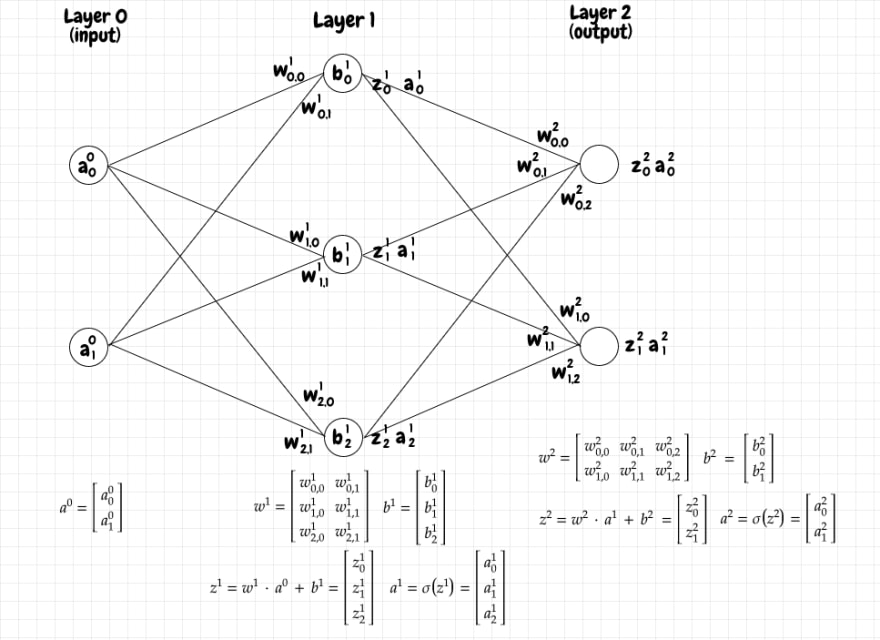
Keep in mind that the superscripts all denote the current layer. They are not exponents.
Since we know that each bias will be updated using a partial derivative, we need to have a partial derivative value corresponding to each bias. Therefore the partial derivative of the cost with respect to the biases in the current layer, ∂C/∂b, should have the same shape as the biases matrix for that layer.
In our example, the output layer has 2 neurons, so the biases matrix, b, for that layer is a 2x1 matrix. Therefore ∂C/∂b for that layer should be a 2x1 matrix as well. From the equations we derived earlier, we know ∂C/∂b requires us to multiply the value of (a-y) and σ'(z). Both of these are 2x1 matrices, so all we need to do is to multiply the value of σ'(z) for each neuron by the difference (a-y) for that same neuron. Intuitively this makes sense: Each value in (a-y) matches up with its corresponding σ'(z) value. When a given value is related to a bunch of incoming or outgoing values, we use the dot product, but here it's a simple 1:1 relationship. This kind of simple product of two identical matrices is called the hadamard product. We represent it as a dot surrounded by a circle. Below is the matrix form of the equation for ∂C/∂b:

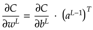
Now let's turn our attention to ∂C/∂w. In our output layer, the weights matrix, w, is a 2x3 matrix. Therefore we want ∂C/∂w to be a 2x3 matrix as well. ∂C/∂w for the current layer is the product of ∂C/∂b for the current layer and the activation matrix a for the previous layer. For our output layer, ∂C/∂b is a 2x1 matrix. a for the previous layer is a 3x1 matrix. We can't multiply a 2x1 and a 3x1 matrix together directly. However, we can transpose a to convert it into a 1x3 matrix! Now the multiplication, using the dot product, produces a 2x3 matrix. That matches up with the shape of w matrix for this layer, so it works. Below is the math notation showing how we obtain ∂C/∂w in matrix form:
Lastly, we need to calculate ∂C/∂aL-1. aL-1 is a 3x1 matrix, so we want ∂C/∂aL-1 to be a 3x1 matrix too. We know that we need to somehow multiply ∂C/∂b against w, the weight matrix for the current layer. ∂C/∂b is a 2x1 matrix and w is a 2x3 matrix. How can we arrange these as a product to obtain a 3x1 matrix? We can first transpose w to get a 3x2 matrix. Now we can take the dot product of wT, a 3x2 matrix, and ∂C/∂b, a 2x1 matrix, which gives us the 3x1 matrix that we want. The equation is in the diagram below:

This last matrix represents the slope of the cost function with respect to the activation in the previous layer. This is very helpful, as we can use this value to calculate the slope with respect to the biases, ∂C/∂b, and weights, ∂C/∂w in that previous layer. Those values can in turn be used to calculate ∂C/∂aL-2, and so on. We continue performing the same operations, layer by layer, until we reach the input layer. Recall that we don't calculate any partial derivatives for the input layer since that's not something that the network adjusts
If you want to build intuition around why we transpose w and then do the dot product, I find it helpful to think of it this way: When we calculate the activation matrix for a given layer, we calculate the dot product of the weight matrix for that layer and the activation matrix from the previous layer. This makes sense, because for each neuron in the next layer, it needs to pull together the weighted activations from all of the neurons in the previous layer. We can think of ∂C/∂aL-1 as the other side of that coin. When we make a small adjustment to the activation of a neuron in the current layer, it will affect the cost function along multiple paths. Let's say we adjust the activation of a single neuron, which connects to 3 neurons in the next layer. We need to add up the effect on the cost function of the sending neuron to the first receiving neuron, the second receiving neuron, and to the third receiving neuron. That will be the first row of our resulting matrix (and so on for each of the other neurons in the sending layer). So, we need to have a matrix where each row represents the cumulative effect of a change in activation by a neuron in the previous layer on each neuron in the next layer.
This method lets us calculate adjustments for the weights and biases in each layer of our network, propagating backward from the output layer. Once that process is done for a given input, we can say that our network has completed a training step. By performing this training for a large number of inputs, we can steadily tune the parameters of our network until it can do cool things like recognizing the mnist images!
The diagram below shows our example network with the partial derivatives for the output layer and middle layer:
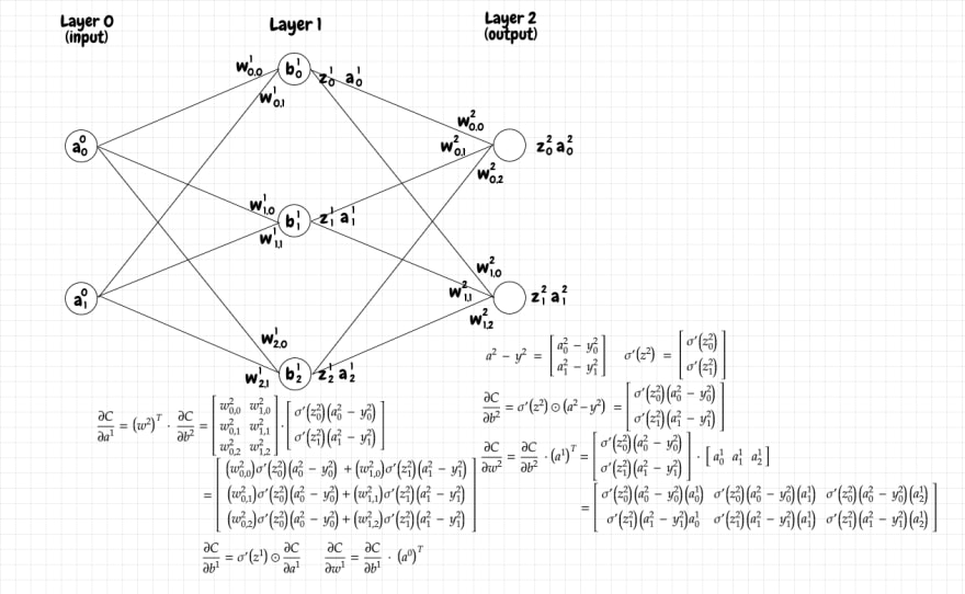
Keep in mind that the superscripts all denote the current layer. They are not exponents.
I've written my own very simple implementation of this neural network in python. I've tried to remove all extraneous details, and to show only the code needed to feed forward the activations, and then to adjust the weights and biases, one training input at a time:
import numpy as np

placeholder = np.array([[]])

class Network:
    def __init__(self, layers, **kw):
        self.num_layers = len(layers)
        self.b = [placeholder]
        self.w = [placeholder]

        if "b" in kw:
            b = kw.get("b")
            self.b += b

        if "w" in kw:
            w = kw.get("w")
            self.w += w

        num_neurons_prev_layer = layers[0]
        for num_neurons_current_layer in layers[1:]:
            if not "b" in kw:
                b = np.random.randn(num_neurons_current_layer, 1)
                self.b.append(b)

            if not "w" in kw:
                w = np.random.randn(num_neurons_current_layer, num_neurons_prev_layer)
                self.w.append(w)

            num_neurons_prev_layer = num_neurons_current_layer

    def feed_forward(self, inputs):
        self.z = [placeholder]
        self.a = [np.asarray([inputs]).transpose()]

        for l in xrange(1, self.num_layers):
            b = self.b[l]
            w = self.w[l]
            a_prev = self.a[l-1]

            z = raw_activation(w, a_prev, b)
            a = sigmoid(z)

            self.z.append(z)
            self.a.append(a)

    def propagate_backward(self, y, step_size):
        y = np.asarray([y]).transpose()

        output_layer = self.num_layers-1
        z = self.z[output_layer]
        a = self.a[output_layer]

        activations_gradient = a - y
        biases_gradient = dc_db(z, activations_gradient)

        a_prev = self.a[output_layer-1]
        weights_gradient = dc_dw(a_prev, biases_gradient)

        w = self.w[output_layer]
        activations_gradient = dc_da_prev(w, biases_gradient)

        self.b[output_layer] -= biases_gradient * step_size
        self.w[output_layer] -= weights_gradient * step_size

        for l in xrange(self.num_layers-2, 0, -1):
            z = self.z[l]
            biases_gradient = dc_db(z, activations_gradient)

            a_prev = self.a[l-1]
            weights_gradient = dc_dw(a_prev, biases_gradient)

            w = self.w[l]
            activations_gradient = dc_da_prev(w, biases_gradient)

            self.b[l] -= biases_gradient * step_size
            self.w[l] -= weights_gradient * step_size

def sigmoid(z):
    return 1.0/(1.0+np.exp(-z))

def sigmoid_prime(z):
    return sigmoid(z)*(1-sigmoid(z))

def raw_activation(w, a, b):
    return np.dot(w,a) + b

def dc_db(z, dc_da):
    return sigmoid_prime(z) * dc_da

def dc_dw(a_prev, dc_db):
    return np.dot(dc_db, a_prev.transpose())

def dc_da_prev(w, dc_db):
    return np.dot(w.transpose(), dc_db)

# demo:
b = [np.array([[0.54001045],
               [0.75958375],
               [0.01870296]]),
     np.array([[-0.32783478],
               [ 0.06061246]])]

w = [np.array([[-0.11499179,  0.454649  ],
               [-0.65801895,  0.56618695],
               [-0.15686814, -0.87499479]]),
     np.array([[ 0.01071228, -0.49139708, -0.81775586],
               [-0.87455946, -0.08351883, -0.77534763]])]

n = Network([2,3,2], b=b, w=w)

inputs = [0.8,0.2]
n.feed_forward(inputs)

y = [0, 1]
n.propagate_backward(y, 0.1)
Note that we normally randomize the initial values of the weights and biases. This is a simple-minded way to create a fairly chaotic initial cost function with ample room for gradient descent. We wouldn't want to risk setting these variables in some predictable way, which might place the cost function into a flat plane from the very start!
Consider that this code is basically sufficient to recognize handwritten images of mnist numbers with a success rate of about 95%! That's quite remarkable. Imagine how much effort it would take to develop a custom algorithm to do the same thing. I think it would be incredibly hard to get to the same level of accuracy that way, but we can achieve pretty good results with the very naive implementation above: All we have are layers of neurons connected together in a completely generic way, with maybe 100 lines of code to perform the forward and backward propagations!
Stochastic Gradient Descent
Adjusting all of the weights and biases for every single input, as in the above code, can be slow. A common speedup technique is to run a batch of inputs through the network and to treat that as a single training step. In other words, first we calculate our partial derivatives for a bunch of randomly selected training inputs. We keep adding the most recent partial derivatives to each gradient matrix. Once we've done that, we divide each of these cumulative partial derivatives by the number of samples in the batch. We then update the weights and biases just once against this average slope. We can then continue doing the same thing with another batch of inputs. This is called stochastic gradient descent. Intuitively, this means our movements down the slope of the landscape are a bit more jerky than they would be otherwise. If we adjusted all of the parameters after every input, our path downward would be a smoother curve, but it would take longer to compute.
MNIST Image Recognition
Michael Nielsen's python code (github)for recognizing mnist images easily reaches approximately a 95% recognition rate after training for just a few minutes on a commodity PC. The following script runs the network with a single hidden layer of 30 neurons (run.py):
import mnist_loader
import network

training_data, validation_data, test_data = mnist_loader.load_data_wrapper()

net = network.Network([784, 30, 10])
net.SGD(training_data, 30, 10, 3.0, test_data=test_data)
The results below show that the network achieves close to 95% accuracy:
C:\Dev\python\neural-networks-and-deep-learning\src>python run.py
Epoch 0: 9032 / 10000
...
Epoch 29: 9458 / 10000
If we change the network to 2 hidden layers of 16 neurons each, like in Grant Sanderson's video (run2.py):
import mnist_loader
import network

training_data, validation_data, test_data = mnist_loader.load_data_wrapper()

net = network.Network([784, 16, 16, 10])
net.SGD(training_data, 30, 10, 3.0, test_data=test_data)
The results seem to be about the same:
C:\Dev\python\neural-networks-and-deep-learning\src>python run2.py
Epoch 0: 8957 / 10000
...
Epoch 29: 9385 / 10000
If we omit the hidden layer completely and just send our input layer directly to the output layer, the accuracy falls quite a bit, down to 75%.
In his video, Grant Sanderson speculates a bit about what the different layers might mean conceptually. He tosses out the idea that the first hidden layer might identify the parts of basic units of handwritten numbers. For example, it might break down an "o" loop into several parts. The second hidden layer might then put these individual parts together, e.g. A 9 might be an "o" loop and a line or curved tail sticking out of it.
However, Grant found that examining the hidden layers didn't reveal anything so clear-cut, just rather noisy data that only shows hints of a pattern. This suggests that this neural network doesn't have to find minima that make sense to us as human beings. It seems to find local minima that are just good enough to do a pretty decent job of solving the problem, but these minima don't fully encapsulate what the numbers mean. That is, as Grant puts it, in the unfathomably large 13,000 dimensional space of weights and biases, our network found itself a happy little local minimum that, despite successfully classifying most images, doesn't exactly pick up on the patterns we might have hoped for... Even if this network can recognize digits pretty well, it has no idea how to draw them. One outcome of this fact is that our particular network will just as confidently classify an image of random pixels as it does a real mnist image!
Our simple network clearly has limitations. For example, the hidden layers don't seem to have any clear pattern or meaning. Also, with large numbers of neurons in each layer, having each of the neurons in one layer connected to all of the neurons in the next layer can become a performance problem. It's also a bit odd after all, isn't it, that all of our input neurons are treated the same, whether they're close together or on opposite sides of the image!
These are issues that are dealt with in some of the more sophisticated approaches to neural networks that have been developed over time. If you'd like to go deeper, check out further developments like deep learning, convolutional neural networks, recurrent neural networks, and LSTM networks. With all that being said, a great thing about the simple network we've worked through in this article is that it can already do something useful and it's pretty easy to understand!

Top comments (0)