
In the world of cybersecurity, a big challenge is figuring out what is and what is not malicious. This is important for all sorts of security tools, like ones that look for hackers, viruses, or flaws in software. Typically, this is done by comparing the incoming attack with a bunch of patterns or rules we already know. But this method isn't always accurate. The rules don't get updated regularly, and sometimes they get mixed up with so many other rules that they can't work properly.
A more accurate solution to this is using artificial intelligence (AI). In today's world of technology, AI has affected almost every industry, if not all, and cybersecurity is not an exception. What stands out in AI is its power to analyse vast amounts of data and detect anomalies as well.
In this tutorial, we will explore the power of AI in analysing vast amounts of data that contain vectors of cyber attacks and teach this AI to distinguish between an attack and normal behaviour.
Prerequsites
To get the most out of this tutorial, you should:
- Have a basic knowledge of Python programming.
- Understand machine learning; i.e., you have built a basic classification or regression model.
- Cultivate curiosity about the application of AI in security.
What is cyber injection?
Cyber injection attacks, also known as code injection attacks, are a prevalent type of cyber threat where malicious code is injected into a system or application to compromise its integrity or steal sensitive information. These attacks can take various forms, including SQL injection, XSS (Cross-Site Scripting), and command injection, among others.
SQL injection involves inserting malicious SQL code into input fields of a web application to manipulate the database or gain unauthorised access to data. XSS attacks inject malicious scripts into web pages, allowing attackers to steal session cookies or redirect users to malicious sites. Command injection attacks exploit vulnerabilities in applications that execute shell commands, enabling attackers to execute arbitrary commands on the server.
Building AI-based cyber injection detector
Detecting cyber injection attacks can be challenging due to their diverse nature and the evolving tactics used by attackers. However, with the advancements in AI and machine learning (ML), detection methods have become more sophisticated. AI algorithms can analyse patterns in network traffic, application behaviour, and system logs to identify anomalies indicative of injection attacks.
ML models trained on historical data can learn to recognise patterns associated with known injection attacks and detect deviations from normal behaviour.
Now that you have an introductory understanding of cyber injection and how AI can assist in detecting it, let's follow these steps to proceed with building this AI.
Step 1: Data Collection.
For this project, we will be using real-world data from past examples of API request vectors. The vector in the dataset denotes data that encapsulates attributes crucial for identifying the presence of an SQL injection attack. Typically, this vector encompasses details regarding the API request, including parameters, headers, or payloads. These components can then be scrutinized by a machine learning model to discern indicators of a SQL injection attack.
You can download this data from kaggle.
The training data from Kaggle is divided into two parts:
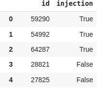
- info.csv: This file contains the type label of each attack vector (i.e., whether a particular vector is an attack or not).
- train.msgpack: This is the main data for this project and will be used to train the machine learning model. It is stored in the messagepack format and contains various types of attack vectors.
Load the train.msgpack:
# Load the data that contains the attack vectors
with open("/content/train.msgpack", "rb") as data_file:  # Open train.msgpack file in binary read mode
    train = msgpack.unpack(data_file)  # Unpack the data using msgpack

# Transforming train data to a pandas DataFrame
train = pd.DataFrame(train)  # Convert unpacked data into a DataFrame
train.columns = ['id', 'vector']  # Rename columns of the DataFrame
train.head()  # Display the first few rows of the DataFrame
Load the info.csv:
# Load data that contains the type label of each attack vector
# (i.e., whether a particular vector is an attack or not)
url_1 = "https://raw.githubusercontent.com/cyberholics/Cyber-Injection-Attack-Detection-With-Machine-Learning/main/Data/info.csv"  # URL of the CSV file containing the attack vector labels
info = pd.read_csv(url_1)  # Reading the CSV file into a pandas DataFrame
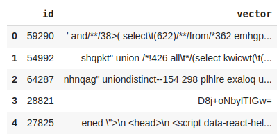
Inspect an example of a vector in the dataset:
# View the data sample to understand the data
train.iloc[2].values  # Retrieve values of the third row in the DataFrame to examine the data sample

The data looks messy, with lots of symbols, strange word formats, and web links. Right now, we're not sure if cleaning it up will help; it might even make things worse. So, let's start with something simple: tokenizing the vectors at the character level.
# View the data sample to understand the data
train.iloc[2].values  # Retrieve values of the third row in the DataFrame to examine the data sample
Step 2: Data preparation
After obtaining the data to build our machine learning model, the next step is to prepare the data. In this data preparation step, we will explore the data as well as convert it to a format that the machine learning algorithm can understand.
The following code will prepare the data.
# Convert the 'vector' column in the train dataset to string type to ensure consistency
train['vector'] = train['vector'].astype(str)

#Initialize the TfidfVectorizer with specified parameters
# ngram_range=(1, 4) specifies that we want to consider uni-grams, bi-grams, tri-grams, and four-grams
# analyzer='char' indicates that we want to tokenize the input text into characters
vectorizer = TfidfVectorizer(ngram_range=(1, 4), analyzer='char')


# Fit the vectorizer on the combined train data to learn the vocabulary and IDF values
vectorizer.fit(list(train['vector'].values))

# Transform the 'vector' column of the train dataset into a sparse matrix representation using the fitted vectorizer
train_vectorized = vectorizer.transform(train['vector'])

# Creating a label input for the model
y = np.array([1 if i == True else 0 for i in info.injection.values])
# Split the data into train and test sets
X_train, X_test, y_train, y_test = train_test_split(train_vectorized, y, test_size=0.2, random_state=42)
Step 3: Building the model
This is the modeling phase of the project, and it's the most eagerly anticipated part for many machine learning practitioners. During this stage, we will train a classification model to learn from the prepared data. For this project, we will utilise the XGBoost model. Now, let's delve into what XGBoost is all about.
XGBoost, short for Extreme Gradient Boosting, is a powerful and popular machine learning algorithm that is highly effective for both regression and classification tasks. It is an implementation of gradient boosting decision trees designed for speed and performance. XGBoost has gained widespread adoption in various machine learning competitions and real-world applications due to its ability to deliver high accuracy and efficiency.
Train the model:
# Define parameters for XGBoost model
params = {
    'max_depth': 6,  # Maximum tree depth
    'eta': 0.1,  # Learning rate
    'objective': 'binary:logistic',  # Binary classification
    'eval_metric': 'auc'  # Evaluation metric: AUC
}

# Convert data into DMatrix
dtrain = xgb.DMatrix(X_train, label=y_train)
dtest = xgb.DMatrix(X_test, label=y_test)

# Train the XGBoost model
num_rounds = 100
xgb_model = xgb.train(params, dtrain, num_rounds)
Evaluate the trained model:
After training the model, we have to evaluate it to see how well it performs. This evaluation helps us determine if the model is generating false positives. The evaluation metric we will use is the Area Under the Curve (AUC) score.
The AUC score is a key metric in binary classification, measuring a model's ability to distinguish between positive and negative instances. It ranges from 0.5 to 1, with higher scores indicating better performance. AUC is especially useful for imbalanced datasets and provides a reliable measure of predictive power.
# Predict probabilities on the test set
preds = xgb_model.predict(dtest)

# Calculate AUC
auc = roc_auc_score(y_test, preds)
print("AUC:", auc)
![]()
We have a 0.99 AUC score. An AUC of 0.99 indicates a very high level of model performance.
Conclusion
Thank you for following this tutorial to the end. Throughout this tutorial, you have learned how to build an AI model capable of detecting cyber attacks. However, building the model is just the beginning. To fully utilise its capabilities, you should take the model to production, where it can be deployed in real-world scenarios.
Deployment methods vary depending on the specific requirements and infrastructure of your organisation. One common approach is deploying the model as a web service or API, allowing it to integrate seamlessly with existing systems. Alternatively, you can deploy the model within containerised environments using platforms like Docker and Kubernetes for scalability and flexibility. Whichever method you choose, ensuring proper monitoring, security, and maintenance of the deployed model is crucial for its effectiveness in real-world applications.
If you have any questions or suggestions, feel free to reach out to me. Your feedback is valuable.


Top comments (0)