Table of Contents

Introduction
Getting started with YOLOv8 segmentation
Train the YOLOv8 model for image segmentation
Using YOLOv8 segmentation model in production
    Export the YOLOv8 segmentation model to ONNX
    Load the model using ONNX
    Prepare the input
    Run the model
    Process the output
        Join bounding boxes and masks
        Parse the combined output
        Process segmentation masks
        Calculate bounding polygons
    Draw bounding polygons on the image
Create a segmentation web application
    Create a backend
    Create a frontend
Conclusion

Introduction

This is the fourth part of my YOLOv8 series. In previous articles, I described how to use the YOLOv8 to detect objects on images and in videos using different programming languages. However, the YOLOv8 also can be used to detect objects more precisely, using instance segmentation.

The result of object detection is a list of bounding boxes around all detected objects. The result of the instance segmentation is a segmentation mask of each detected object. The segmentation mask is a black-white image on which all pixels that belong to the object are white, and all other pixels are black, as displayed on the next image:

After having this mask, which is, in fact, a 2D array with values either 0 for background pixels and 255 for object pixels, you can apply it to the image to draw only pixels of the image that displayed as white on the mask. This way you can, for example, remove background from the image:

and set new background for objects:

The same way, you can run instance segmentation for each frame in video and remove background from the whole video.

Furthermore, having these bit masks of detected objects, you can calculate their contours.

The calculated contour is a polygon, which is an array of point coordinates. This polygon can be used to identify the detected objects on images in real world applications much more precisely than just using the bounding boxes.

The instance segmentation used in self-driving cars, medical imagining, aerial crop monitoring, and more.

For example, the well known ChromaCam application and its analogues use image segmentation to detect your shape and boundaries and replace or blur background around you while you stream a video from a web camera.

In this article, I will guide you how to implement instance segmentation for images using YOLOv8. First, we will use default Ultralytics API where most of internal work greatly automated, and we will use a pretrained model shipped with YOLOv8 that detects 80 objects classes from the COCO dataset. Then I will give a review how to prepare data and train the model on it to detect custom object classes, that can be required for specific business tasks. Then, after using high level API, we will dive to the internals and will prepare the input for the YOLOv8 model and will parse its output by hands. Finally, we will create a web application in which you can upload the image, pass it through the YOLOv8 model and display contours of all objects, detected on it.

The YOLOv8 segmentation models are based on object detection models, that I covered in previous articles. When you do instance segmentation, the model automatically does object detection and returns both results of object detection and instance segmentation. That is why, it crucially important to read my previous articles of this series, at least first and second parts, because I will reuse a big amount of code from these posts.

Getting started with YOLOv8 segmentation

Let's just start coding. You need an environment where you can run Python code. I recommend to use Jupyter Notebook. In the next sections, all code samples and output assumes that you run this in the Jupyter Notebook.

Ensure that the Ultralytics package installed by running the following command in notebook:

!pip install ultralytics

Then, import the YOLO models factory object:

from ultralytics import YOLO

Then, you need to instantiate the model, that will be used for predictions. I will use a pretrained medium-sized model, shipped with YOLOv8, that can detect 80 object classes. In contrast with object-detection models, the segmentation model names have -seg suffix. So, if you need to load a medium-sized model for segmentation, you need to specify yolov8m-seg.pt file.

model = YOLO("yolov8m-seg.pt")

Also, all the same models for segmentation available: yolov8n-seg.pt, yolov8s-seg.pt, yolov8m-seg.pt, yolov8t-seg.pt and yolov8x-seg.pt.

For all examples, I will use the image with cat and dog, that named cat_dog.jpg and located in the current folder with the notebook:

Let's run the model to get segmentation results for this image:

results = model.predict("cat_dog.jpg")

The predict method for segmentation model works the same as for object detection model. It returns an array of results for each image, specified in the method call. In this case, this array contains a single item. Let's get it:

result = results[0]

Furthermore, the segmentation model runs object detection as well. Consequently, the returned result is almost the same as it was when we ran object detection in the first article of this series. In addition, it has the masks property, which is an array of detected object segmentation masks.

Let's see how many masks detected:

masks = result.masks
len(masks)

2

The result is predictable, it segmented 2 objects: dog and cat. Let's get the first of these masks:

mask1 = masks[0]

Each mask is an object that has a set of properties. We will use two of them:

• data - the segmentation mask of the object, which is a black and white image matrix, in which 0 elements are black pixels and 1 elements are white pixels.
• xy - the polygon of object, which is an array of points.

There are other properties exist. All them you can learn in the official documentation

The data property wrapped to PyTorch tensor array, but, I think, it will be more common to work with it as with NumPy array. Let's extract the mask and the polygon:

mask = mask1.data[0].numpy()
polygon = mask1.xy[0]

Let's display the mask of the first object. We will use the Pillow Image object for it. It has the fromarray method to load images from NumPy matrices. Ensure that the Pillow installed:

!pip install pillow

and create an image from the mask:

from PIL import Image
mask_img = Image.fromarray(mask,"I")
mask_img

It should display the following image:

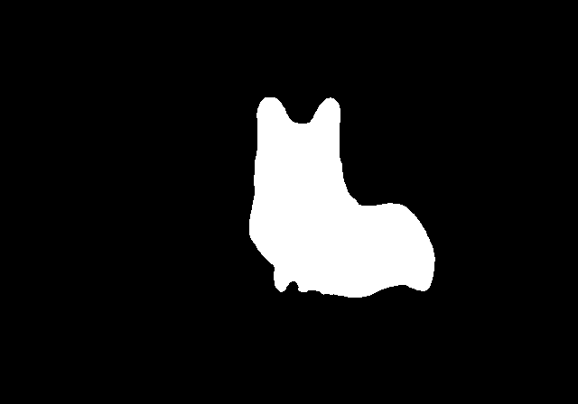So, you see that this is a segmentation mask of the dog.

Now, let's work with polygon object. Display it to see the array of points:

polygon

array([[     280.18,      96.575],
       [      275.4,      101.36],
       [      275.4,      102.31],
       [     274.44,      103.27],
       [     274.44,      105.18],
       [     273.49,      106.14],
       [     273.49,      107.09],
       [     272.53,      108.05],
       [     272.53,      111.87],
       [     271.57,      112.83],
       [     271.57,      117.61],
       [     272.53,      118.57],
       [     272.53,      152.04]
...
       [     302.17,      112.83],
       [     302.17,      110.92],
       [     301.22,      109.96],
       [     301.22,      108.05],
       [     298.35,      105.18],
       [     298.35,      104.22],
       [     297.39,      103.27],
       [     297.39,      102.31],
       [     292.61,      97.531],
       [     291.66,      97.531],
       [      290.7,      96.575]], dtype=float32)

Each point is a list with coordinates [x,y]. You can do whatever you want with it. For example, you can draw it on top of the cat_dog image:

from PIL import ImageDraw

img = Image.open("cat_dog.jpg")
draw = ImageDraw.Draw(img)
draw.polygon(polygon,outline=(0,255,0), width=5)
img

This code imports the ImageDraw module from Pillow that used to draw on top of images. Then, it opens the cat_dog.jpg image and initializes the draw object with it. Then it draws the polygon on it, using the polygon points. The outline argument specifies the line color (green) and the width specifies the line width. Finally, you should see the image with outlined dog:

Now, to summarize this, let's do the same for the second mask:

mask2 = masks[1]
mask = mask2.data[0].numpy()
polygon = mask2.xy[0]
mask_img = Image.fromarray(mask,"I")
mask_img

draw.polygon(polygon,outline=(0,255,0), width=5)
img

For convenience, you can see the whole coding session of this chapter as a video.

Using the models pretrained on well-known objects is ok to start, but in practice, you may need a solution to segment specific objects for a concrete business problem.

For example, someone may need to detect specific products on supermarket shelves or discover brain tumors on x-rays. It's highly likely that this information is not available in public datasets, and there are no free models that know about everything.

So, you have to teach your own model to detect these types of objects. To do that, you need to create a database of annotated images for your problem and train the model on these images.

Train the YOLOv8 model for image segmentation

To train the model, you need to prepare annotated images and split them to training and validation datasets. The training set will be used to teach the model and the validation set will be used to test the results of this study, to measure the quality of the trained model. You can put 80% of images to the training set and 20% to the validation set.

These are the steps that you need to follow to create each of the datasets:

1. Decide and encode classes of objects you want to teach your model to detect. For example, if you want to detect only cats and dogs, then you can state that "0" is cat and "1" is dog.

2. Create a folder for your dataset and two subfolders in it: "images" and "labels".

3. Put the images to the "images" subfolder. The more images you collect, the better for training.

4. For each image, create an annotation text file in the "labels" subfolder. Annotation text files should have the same names as image files and the ".txt" extensions. In annotation file you should add records about each object, that exist on the appropriate image in the following format:
   

{object_class_id} {polygon}

• object_class_id is a label of object class, like for example 0 if it's cat or 1 if it's dog.
• polygon is a coordinates of bounding polygon for this object in the following format: x1 y1 x2 y2 ...

Actually, this is the most time-consuming manual work in a machine learning process: to measure coordinates of bounding polygons for all objects and add them to annotation files. Moreover, coordinates should be normalized to fit in a range from 0 to 1. To calculate them, you need to use the following formulas:

x = x/image_width
y = y/image_height

So, if you have a point with (100,100) coordinate and the image size is (612,415), then, use the following to calculate this point for annotation:

x = 100/612 = 0.163666121
y = 100/415 = 0.240963855

This way, you need to set up polygons for all objects on each image. For example, if you have an image with the following cat and dog polygons:

then you need to create the following annotation file for it:

1 0.45781 0.23271 0.45 0.24423 0.45 0.24654 0.44844 0.24884 0.44844 0.25345 0.44687 0.25575 0.44687 0.25806 0.44531 0.26036 0.44531 0.26958 0.44375 0.27188 0.44375 0.2834 0.44531 0.28571 0.44531 0.36636 0.44375 0.36866 0.44375 0.38018 0.44219 0.38248 0.44219 0.3894 0.44062 0.3917 0.44062 0.42857 0.43906 0.43087 0.43906 0.45622 0.44062 0.45852 0.44062 0.48157 0.43906 0.48387 0.43906 0.49309 0.4375 0.49539 0.4375 0.50461 0.43594 0.50691 0.43594 0.51843 0.43437 0.52074 0.43437 0.52765 0.43281 0.52995 0.43281 0.54148 0.43125 0.54378 0.43125 0.58295 0.43281 0.58526 0.43281 0.58986 0.43437 0.59217 0.43437 0.59447 0.4375 0.59908 0.4375 0.60139 0.44219 0.6083 0.44219 0.6106 0.44375 0.61291 0.44375 0.61521 0.44531 0.61752 0.44531 0.61982 0.45156 0.62904 0.45156 0.63134 0.46875 0.65669 0.47031 0.65669 0.47344 0.6613 0.47344 0.6636 0.475 0.6659 0.475 0.67512 0.47344 0.67742 0.47344 0.69816 0.475 0.70047 0.475 0.71199 0.47656 0.71429 0.47656 0.7166 0.48437 0.72812 0.4875 0.72812 0.48906 0.72581 0.49062 0.72581 0.49375 0.7212 0.49375 0.7166 0.49844 0.70968 0.49844 0.70738 0.50156 0.70277 0.50312 0.70277 0.50469 0.70047 0.50937 0.70047 0.51406 0.70738 0.51406 0.70968 0.51562 0.71199 0.51562 0.71429 0.51719 0.7166 0.51562 0.7189 0.51562 0.72351 0.51719 0.72581 0.51875 0.72581 0.52031 0.72812 0.52969 0.72812 0.53281 0.72351 0.54531 0.72351 0.54687 0.72581 0.55156 0. 72581 0.55625 0.73273 0.55781 0.73273 0.55937 0.73503 0.56094 0.73273 0.56875 0.73273 0.57031 0.73503 0.575 0.73503 0.57656 0.73273 0.57812 0.73503 0.58281 0.73503 0.58437 0.73733 0.59375 0.73733 0.59531 0.73964 0.6 0.73964 0.60156 0.74194 0.625 0.74194 0.62656 0.73964 0.63281 0.73964 0.63437 0.73733 0.63906 0.73733 0.64062 0.73503 0.64219 0.73503 0.64375 0.73273 0.64531 0.73273 0.64687 0.73042 0.64844 0.73042 0.65 0.72812 0.65156 0.72812 0.65312 0.72581 0.65469 0.72581 0.65625 0.72351 0.65781 0.72351 0.65937 0.7212 0.6625 0.7212 0.66406 0.7189 0.66719 0.7189 0.66875 0.7166 0.67187 0.7166 0.67344 0.71429 0.67969 0.71429 0.68125 0.71199 0.6875 0.71199 0.68906 0.70968 0.70156 0.70968 0.70312 0.71199 0.70469 0.71199 0.70781 0.7166 0.71094 0.7166 0.7125 0.7189 0.71562 0.7189 0.71719 0.7212 0.71875 0.7212 0.72031 0.72351 0.72656 0.72351 0.72812 0.72581 0.73437 0.72581 0.73594 0.72351 0.7375 0.72351 0.74219 0.7166 0.74219 0.71429 0.74375 0.71199 0.74375 0.70738 0.74531 0.70508 0.74531 0.70047 0.74687 0.69816 0.74687 0.69125 0.74844 0.68895 0.74844 0.67742 0.75 0.67512 0.75 0.65208 0.75156 0.64977 0.75156 0.64056 0.75 0.63825 0.75 0.62904 0.74844 0.62673 0.74844 0.61752 0.74687 0.61521 0.74687 0.6106 0.74531 0.6083 0.74531 0.60599 0.74375 0.60369 0.74375 0.60139 0.74219 0.59908 0.74219 0.59447 0.74062 0.59217 0.74062 0.58986 0.7375 0.58526 0.7375 0.58065 0.73594 0.57834 0.73594 0.57373 0.73281 0.56913 0.73281 0.56682 0.72969 0.56221 0.72969 0.55991 0.72812 0.55761 0.72812 0.5553 0.725 0.55069 0.725 0.54839 0.72031 0.54148 0.72031 0.53917 0.71562 0.53226 0.71562 0.52995 0.71406 0.52995 0.70156 0.51152 0.7 0.51152 0.69844 0.50922 0.69687 0.50922 0.69531 0.50691 0.69219 0.50691 0.69062 0.50461 0.67969 0.50461 0.67812 0.5023 0.67031 0.5023 0.66875 0.50461 0.66094 0.50461 0.65937 0.50691 0.65156 0.50691 0.65 0.50922 0.625 0.50922 0.62344 0.50691 0.62031 0.50691 0.61875 0.50461 0.61875 0.5023 0.61562 0.4977 0.61562 0.49539 0.6125 0.49078 0.61094 0.49078 0.60312 0.47926 0.60312 0.47696 0.6 0.47235 0.6 0.46774 0.59844 0.46544 0.59844 0.46083 0.59687 0.45852 0.59687 0.45392 0.59531 0.45161 0.59531 0.44931 0.59375 0.447 0.59375 0.44009 0.59219 0.43779 0.59219 0.42396 0.59062 0.42166 0.59062 0.40092 0.58906 0.39861 0.58906 0.39631 0.5875 0.39401 0.5875 0.38709 0.58594 0.38479 0.58594 0.29723 0.5875 0.29492 0.5875 0.26036 0.58594 0.25806 0.58594 0.25114 0.58437 0.24884 0.58437 0.24654 0.57656 0.23502 0.57344 0.23502 0.57187 0.23271 0.57031 0.23271 0.56875 0.23502 0.56406 0.23502 0.55156 0.25345 0.55156 0.25575 0.55 0.25806 0.55 0.26036 0.54844 0.26267 0.54844 0.26497 0.54531 0.26958 0.54531 0.27188 0.54375 0.27419 0.54375 0.27649 0.54219 0.2788 0.54219 0.2834 0.5375 0.29032 0.5375 0.29262 0.53437 0.29723 0.53125 0.29723 0.52969 0.29953 0.51562 0.29953 0.51406 0.29723 0.50937 0.29723 0.50781 0.29492 0.50625 0.29492 0.49844 0.2834 0.49844 0.2811 0.49687 0.2788 0.49687 0.27649 0.49375 0.27188 0.49375 0.26727 0.49219 0.26497 0.49219 0.26036 0.4875 0.25345 0.4875 0.25114 0.48594 0.24884 0.48594 0.24654 0.47812 0.23502 0.47656 0.23502 0.475 0.23271
0 0.25 0.41705 0.24844 0.41935 0.24687 0.41935 0.24531 0.42166 0.24531 0.42857 0.24375 0.43087 0.24375 0.46774 0.24219 0.47005 0.24219 0.48157 0.24062 0.48387 0.24062 0.48848 0.23906 0.49078 0.23906 0.4977 0.2375 0.5 0.2375 0.50922 0.23594 0.51152 0.23594 0.52074 0.23437 0.52304 0.23437 0.52995 0.23281 0.53226 0.23281 0.54378 0.23125 0.54608 0.23125 0.63825 0.23281 0.64056 0.23281 0.65208 0.23437 0.65438 0.23437 0.65669 0.23594 0.65899 0.23594 0.6636 0.2375 0.6659 0.2375 0.67512 0.23906 0.67742 0.23906 0.68434 0.24062 0.68664 0.24062 0.69125 0.24219 0.69355 0.24219 0.70047 0.24375 0.70277 0.24375 0.70968 0.24531 0.71199 0.24531 0.7166 0.25 0.72351 0.25 0.72581 0.25156 0.72812 0.25625 0.72812 0.25781 0.73042 0.2875 0.73042 0.28906 0.73273 0.29219 0.73273 0.29375 0.73503 0.29687 0.73503 0.29844 0.73733 0.30312 0.73733 0.30469 0.73964 0.30781 0.73964 0.30937 0.74194 0.3125 0.74194 0.31406 0.74425 0.31562 0.74425 0.31875 0.74886 0.32031 0.74886 0.32187 0.75116 0.32344 0.75116 0.325 0.75346 0.3375 0.75346 0.33906 0.75116 0.35312 0.75116 0.35469 0.75346 0.36094 0.75346 0.3625 0.75577 0.37031 0.75577 0.37187 0.75807 0.37812 0.75807 0.37969 0.75577 0.38594 0.75577 0.3875 0.75346 0.40781 0.75346 0.4125 0.74655 0.4125 0.74425 0.41562 0.73964 0.41562 0.7166 0.41406 0.71429 0.41406 0.71199 0.40937 0.70508 0.40937 0.70277 0.40469 0.69586 0.40469 0.68895 0.40312 0.68664 0.40312 0.67742 0.40156 0.67512 0.40156 0.66821 0.4 0.6659 0.4 0.6106 0.39844 0.6083 0.39844 0.59447 0.39687 0.59217 0.39687 0.58756 0.39531 0.58526 0.39531 0.58295 0.39375 0.58065 0.39375 0.57604 0.39219 0.57373 0.39219 0.57143 0.39062 0.56913 0.39062 0.56682 0.38906 0.56452 0.38906 0.56221 0.3875 0.55991 0.3875 0.55761 0.38594 0.5553 0.38594 0.55069 0.38437 0.54839 0.38437 0.54608 0.38125 0.54148 0.38125 0.53917 0.37812 0.53456 0.37812 0.53226 0.36875 0.51843 0.36719 0.51843 0.36406 0.51383 0.3625 0.51383 0.35937 0.50922 0.35781 0.50922 0.35625 0.50691 0.35312 0.50691 0.35 0.5023 0.34844 0.5023 0.34687 0.5 0.34375 0.5 0.34219 0.4977 0.34062 0.4977 0.33125 0.48387 0.33125 0.47926 0.32969 0.47696 0.32969 0.46083 0.33125 0.45852 0.33125 0.447 0.33281 0.4447 0.33281 0.42396 0.33437 0.42166 0.33281 0.41935 0.32969 0.41935 0.32812 0.41705 0.32656 0.41705 0.325 0.41935 0.32187 0.41935 0.31875 0.42396 0.31719 0.42396 0.30937 0.43548 0.30781 0.43548 0.30625 0.43779 0.30469 0.43779 0.30312 0.44009 0.29687 0.44009 0.29531 0.44239 0.29219 0.44239 0.29062 0.44009 0.27656 0.44009 0.27344 0.43548 0.27187 0.43548 0.26719 0.42857 0.26719 0.42627 0.26562 0.42396 0.26406 0.42396 0.2625 0.42166 0.2625 0.41935 0.26094 0.41935 0.25937 0.41705

The first line defines normalized polygon for dog (class_id=1) and the second line defines normalized polygon for cat (class_id=0).

After adding and annotating all images, the dataset is ready. You need to create two datasets and place them in different folders. The final folder structure can look like this:

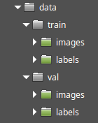Here the training dataset located in the "train" folder and the validation dataset located in the "val" folder.

Finally, you need to create a dataset descriptor YAML-file, that points to created datasets and describes the object classes in them. This is a sample of this file for the data, created above:

train: ../train/images
val: ../val/images

nc: 2
names: ['cat','dog']

In the first two lines, you need to specify paths to the images of the training and the validation datasets. The paths can be either relative to the current folder or absolute. Then, the nc line specifies the number of classes that exist in these datasets and the names is an array of class names in correct order. Indexes of these items are numbers that you used when annotated the images, and these indexes will be returned by the model when detect objects using the predict method. So, if you used "0" for cats, then it should be the first item in the names array.

This YAML file should be passed to the train method of the model to start a training process.

To make this process easier, there are a lot of programs exist to visually annotate images for machine learning. You can ask a search engine something like "software to annotate images for machine learning" to get a list of them. There are also many online tools that can do all this work. One of the great online tools for this is the Roboflow Annotate. Using this service, you just need to upload your images, draw polygons on them, and set class for each polygon. Then, the tool will automatically create annotation files, split your data to train and validation datasets, will create a YAML descriptor file, and then you can export and download the annotated data as a ZIP file.

In the next video, I show how to use the Roboflow to create the "cats and dogs" micro-dataset.

This example has just two images, but for real life problems, that database should be much bigger. To train a good model, you should have hundreds of annotated images.

Also, when prepare images database, try to make it balanced. It should have an equal number of objects of each class, e.g. equal number of dogs and cats. Otherwise, the model trained on it could predict one class better than another.

After the data is ready, copy it to the folder with your Python code.

The training process for image segmentation is exactly the same as for object detection. You can read about this in the appropriate section of the first article of this series.

After you have trained model in the best.pt file, you can use it to predict segmentation masks and polygons of your specific object classes.

Using YOLOv8 segmentation model in production

For all the job, we used the Ultralytics high level APIs, provided with YOLOv8 package by default. These APIs are based on the PyTorch framework, that used to create the bigger part of neural networks today. It's quite convenient on the one hand, but dependence on these high level APIs has a negative effect as well. If you need to run the app created this way in production, you should install all this environment there, including Python, PyTorch and many other dependencies. To run this on a clean new server, you'll need to download and install more than 1 GB of third party libraries!! This is definitely not a way to go. Also, what if you do not have Python in your production environment? What if all your other code written on other programming language, and you do not plan to use Python? Or what if you want to run the model on a mobile phone on Android or iOS?

Using Ultralytics packages is great for experimenting, training and preparing the models for production. However, in production itself, you should get rid of these high-level APIs. You have to load and use the model directly. To do this, you need to understand how the YOLOv8 neural network works under the hood and write more code to provide input to the model and to process the output from it. As a reward, you will get an opportunity to make your apps tiny and fast, you will not need to have PyTorch installed to run them.

Export the YOLOv8 segmentation model to ONNX

Run the following code to export the YOLOv8 segmentation model to ONNX:

model = YOLO("yolov8m-seg.pt")
model.export(format="onnx")

This code should create the yolov8m-seg.onnx file, which is an ONNX version of middle-sized YOLOv8 segmentation model. Let's discover how to make predictions using the ONNX API, instead of Ultralytics.

Load the model using ONNX

Now when you have a model, let's use ONNX to work with it. Install the ONNX runtime library for Python by running the following command in your Jupyter notebook:

!pip install onnxruntime

and import it:

import onnxruntime as ort

We set the ort alias to it. The ort module is a root of the ONNX API. The main object of this API is the InferenceSession which used to instantiate a model to run prediction on it. Model instantiation works very similar to what we did before with Ultralytics:

model = ort.InferenceSession("yolov8m-seg.onnx")

Here we loaded the model, but from ".onnx" file instead on ".pt". And now it's ready to run.

Before continue reading, remember the appropriate section of the article, where we used the YOLOv8 ONNX model for object detection, because image segmentation model does object detection as well and many things are similar, and some thorough descriptions will be omitted here. We will go through the same steps as there: prepare the input, run the model and process the output to finally get segmentation masks and bounding polygons for all detected objects.

Prepare the input

Let's see, which inputs this model expects to receive and which outputs it will produce.

inputs = model.get_inputs()
len(inputs)

1

This code showed that the model expects to get a single input. Now let's display the information about this input:

input = inputs[0]

print("Name: ",input.name)
print("Shape: ",input.shape)
print("Type: ",input.type)

Name:  images
Shape:  [1, 3, 640, 640]
Type:  tensor(float)

As you see, the input is the same as for the object detection model. It's a 3-channel image of 640x640 pixels. Let's prepare it the same way, using the Pillow module to load the image:

from PIL import Image
import numpy as np

img = Image.open("cat_dog.jpg")

# save original image size for future
img_width, img_height = img.size;
# convert image to RGB,
img = img.convert("RGB");
# resize to 640x640
img = img.resize((640,640))

# convert the image to tensor 
# of [1,3,640,640] as required for 
# the model input
input = np.array(img)
input = input.transpose(2,0,1)
input = input.reshape(1,3,640,640).astype('float32')
input = input/255.0

So, we have the input, which can be passed through the model.

Run the model

Let's discover, which outputs the model will produce before running it:

outputs = model.get_outputs()
len(outputs)

2

Here you can see something different. This model produces two outputs instead of a single one, as it was for object detection. Let's print information about each of these outputs:

for output in outputs:
    print("Name: ", output.name)
    print("Shape: ", output.shape)
    print("Type: ", output.type)

Name:  output0
Shape:  [1, 116, 8400]
Type:  tensor(float)
---
Name:  output1
Shape:  [1, 32, 160, 160]
Type:  tensor(float)
---

As previously said, the segmentation model outputs both object detection bounding boxes and segmentation masks.

• output0 - contains detected bounding boxes and object classes, the same as for object detection
• output1 - contains segmentation masks for detected objects. There are only raw masks and no polygons.

Let's run the model to receive these outputs:

outputs = model.run(None, {"images":input})
len(outputs)

2

Now you have these two outputs and it's time to process them.

Process the output

The model returned 2 outputs. Let's define them for convenience and show their shapes:

output0 = outputs[0]
output1 = outputs[1]
print("Output0:",output0.shape,"Output1:",output1.shape)

Output0: (1, 116, 8400) Output1: (1, 32, 160, 160)

The output0 tensor is close to the same, that we got for the object detection in the previous article.

output0 = output0[0].transpose()
output1 = output1[0]
print("Output0:",output0.shape,"Output1:",output1.shape)

Output0: (8400, 116) Output1: (32, 160, 160)

The output0 contains 8400 detected objects (most of them are garbage), however, each of them has 116 parameters instead of 84. This is because it contains additional 32 parameters for segmentation masks. This output includes the same 84 parameters of the object detection model and 32 segmentation masks. That is why, you need to split this input to two parts:

boxes = output0[:,0:84]
masks = output0[:,84:]
print("Boxes:",boxes.shape,"Masks:",masks.shape)

Boxes: (8400, 84) Masks: (8400, 32)

Keep in mind, that if you use a custom trained model, the number of classes could be not 80, but other number. In this case you need to use the (number of classes)+4 to split output to boxes and masks, not 84.

Join bounding boxes and masks

The boxes matrix you can process the same way as for object detection.

The data in the masks matrix is not enough to produce segmentation masks. You need to join it with the second output somehow. Let's print the masks and the output1 shapes close to each other to see how to join them:

print(masks.shape,output1.shape)

(8400, 32) (32, 160, 160)

Do you see that the number of columns of first matrix is the same as the number of rows in second one? It means that you can multiply these matrices to join them together. After joining them, you could receive something like (8400,160,160). These are segmentation masks for all detected boxes. Each segmentation mask has 160x160 size.

However, to make matrix multiplication you need to reshape the output1 to have the same number of dimensions:

output1 = output1.reshape(32,160*160)
print(masks.shape,output1.shape)

(8400, 32) (32, 25600)

Later you will need to reshape 25600 to 160,160.

Now it's clear that you can do matrix multiplication. The @ operator from NumPy library used for this:

masks = masks @ output1
print(masks.shape)

(8400, 25600)

So, now you have 8400 detected boxes and segmentation masks for them:

print(boxes.shape,masks.shape)

(8400, 84) (8400, 25600)

Now we will connect them together. Let's add 25600 columns from the second matrix to the first one:

boxes = np.hstack((boxes,masks))
print(boxes.shape)

(8400, 25684)

The hstack function connects two 2D NumPy arrays horizontally by appending columns from the second array to the right of the first array. Finally, for each detected object, we have the following columns:

• 0-4 - x_center, y_center, width and height of bounding box
• 4-84 - Object class probabilities for all 80 classes, that this YOLOv8 model can detect
• 84-25684 - Pixels of segmentation mask as a single row. Actually, the segmentation mask is a 160x160 matrix, but we just flattened it.

Parse the combined output

Now nothing can stop you from parsing this matrix. For everything except segmentation mask, you can reuse the same code from the appropriate section of previous article. Let's copy-paste required functions and definitions from there:

yolo_classes = [
    "person", "bicycle", "car", "motorcycle", "airplane", "bus", "train", "truck", "boat",
    "traffic light", "fire hydrant", "stop sign", "parking meter", "bench", "bird", "cat", "dog", "horse",
    "sheep", "cow", "elephant", "bear", "zebra", "giraffe", "backpack", "umbrella", "handbag", "tie",
    "suitcase", "frisbee", "skis", "snowboard", "sports ball", "kite", "baseball bat", "baseball glove",
    "skateboard", "surfboard", "tennis racket", "bottle", "wine glass", "cup", "fork", "knife", "spoon",
    "bowl", "banana", "apple", "sandwich", "orange", "broccoli", "carrot", "hot dog", "pizza", "donut",
    "cake", "chair", "couch", "potted plant", "bed", "dining table", "toilet", "tv", "laptop", "mouse",
    "remote", "keyboard", "cell phone", "microwave", "oven", "toaster", "sink", "refrigerator", "book",
    "clock", "vase", "scissors", "teddy bear", "hair drier", "toothbrush"
]

def intersection(box1,box2):
    box1_x1,box1_y1,box1_x2,box1_y2 = box1[:4]
    box2_x1,box2_y1,box2_x2,box2_y2 = box2[:4]
    x1 = max(box1_x1,box2_x1)
    y1 = max(box1_y1,box2_y1)
    x2 = min(box1_x2,box2_x2)
    y2 = min(box1_y2,box2_y2)
    return (x2-x1)*(y2-y1)

def union(box1,box2):
    box1_x1,box1_y1,box1_x2,box1_y2 = box1[:4]
    box2_x1,box2_y1,box2_x2,box2_y2 = box2[:4]
    box1_area = (box1_x2-box1_x1)*(box1_y2-box1_y1)
    box2_area = (box2_x2-box2_x1)*(box2_y2-box2_y1)
    return box1_area + box2_area - intersection(box1,box2)

def iou(box1,box2):
    return intersection(box1,box2)/union(box1,box2)

Now let's traverse the array of detected objects, parse and filter it:

# stub of mask parsing function
def get_mask(row,box):
    mask = row.reshape(160,160)
    return mask

# parse and filter detected objects
objects = []
for row in boxes:
    prob = row[4:84].max()
    if prob < 0.5:
        continue
    xc,yc,w,h = row[:4]
    class_id = row[4:84].argmax()
    x1 = (xc-w/2)/640*img_width
    y1 = (yc-h/2)/640*img_height
    x2 = (xc+w/2)/640*img_width
    y2 = (yc+h/2)/640*img_height
    label = yolo_classes[class_id]
    mask = get_mask(row[84:25684],(x1,y1,x2,y2))
    objects.append([x1,y1,x2,y2,label,prob,mask])

# apply non-maximum suppression to filter duplicated
# boxes
objects.sort(key=lambda x: x[5], reverse=True)
result = []
while len(objects)>0:
    result.append(objects[0])
    objects = [object for object in objects if iou(object,objects[0])<0.7]

print(len(result))

2

If you read that article, then everything except get_mask should be clear here. Finally, it returns 2 detected objects, as this should be for our image.

Process segmentation masks

On the current stage, the get_mask function just reshapes the mask to 160x160 pixels matrix, but it's not a complete mask parsing code. To write correct code in this function, let's get some mask from the result and explore what is it:

mask = result[0][6]
print(mask)

[[    -1.6534     -3.0664     -3.1947 ...     -7.4953     -6.7599     -5.0995]
 [     -2.258     -4.9611     -5.2562 ...     -9.0785     -8.8663     -7.7189]
 [    -2.6319     -5.4276     -5.5777 ...     -8.7668     -8.7555     -8.0009]
 ...
 [    -3.0467     -4.2886     -4.1702 ...     -5.1899     -5.0957     -4.4152]
 [    -3.0335     -4.4031     -4.4115 ...     -5.3815     -5.2315     -4.4424]
 [    -2.7506     -4.1725     -4.3196 ...      -4.692     -4.4167     -3.5068]]

This code printed the mask of the first detected object. The value for each pixel is a weird number. Actually, each of this number should be probability that this pixel belongs to the object. If the probability is low, then this pixel is a background and this pixel should be black, otherwise it should be white. But this is a raw output from neural network and these values should be converted to probabilities. We will use the sigmoid function for this:

This function can return only values in a range from 0 to 1 for any input argument z. This is how you can define it on Python:

def sigmoid(z):
    return 1 / (1 + np.exp(-z))

and apply it to the mask

mask = sigmoid(mask)
print(mask)

[[    0.16065    0.044514    0.039364 ...  0.00055536    0.001158   0.0060625]
 [    0.09466   0.0069568   0.0051882 ...  0.00011408  0.00014104  0.00044417]
 [   0.067116   0.0043745   0.0037671 ...   0.0001558  0.00015757  0.00033503]
 ...
 [   0.045361    0.013539    0.015214 ...   0.0055419   0.0060856    0.011948]
 [   0.045937    0.012091    0.011991 ...   0.0045797   0.0053169    0.011631]
 [   0.060052     0.01518     0.01313 ...   0.0090851     0.01193     0.02912]]

Now you have probabilities for each pixel, and it's time to convert probabilities to real colors. Let's say that if probability less or equal to 0.5, then it will be black color (color 0) and if probability is greater, then it will be white color (color 255).

mask = (mask > 0.5).astype('uint8')*255

• (mask > 0.5) creates a new boolean matrix of the same size in which all items that greater than 0.5 will be True and all elements below 0.5 will be False
• .astype('uint8') converts these values to integers: False to 0 and True to 1
• *255 used to set 255 for all ones to make these pixels white.

Now, this is a real 160x160 image array, in which all pixels that belong to object are white and all pixels that belong to background are black. You can create the Pillow image from this array and display it:

img_mask = Image.fromarray(mask,"L")
img_mask

However, it displays the segmentation mask of the whole image, but we need the mask of only the first detected object. Let's crop it.

Get the coordinates of the object's bounding box first:

x1,y1,x2,y2 = result[0][:4]

Then, keep in mind that the size of mask is 160x160, but the coordinates of the bounding box calculated for real image size, so you need to scale them to the coordinates of mask:

mask_x1 = round(x1/img_width*160)
mask_y1 = round(y1/img_height*160)
mask_x2 = round(x2/img_width*160)
mask_y2 = round(y2/img_height*160)

then crop the mask using them, convert to image again and display it:

mask = mask[mask_y1:mask_y2,mask_x1:mask_x2]

img_mask = Image.fromarray(mask,"L")
img_mask

The last step is to scale this mask to the size of the bounding box of this object.

img_mask = img_mask.resize((round(x2-x1),round(y2-y1)))
img_mask

and convert this final image back to the mask array:

mask = np.array(img_mask)

Now, you can copy all the mask processing code to the get_mask function:

def get_mask(row,box):    
    mask = row.reshape(160,160)
    mask = sigmoid(mask)
    mask = (mask > 0.5).astype('uint8')*255
    x1,y1,x2,y2 = box
    mask_x1 = round(x1/img_width*160)
    mask_y1 = round(y1/img_height*160)
    mask_x2 = round(x2/img_width*160)
    mask_y2 = round(y2/img_height*160)
    mask = mask[mask_y1:mask_y2,mask_x1:mask_x2]
    img_mask = Image.fromarray(mask,"L")
    img_mask = img_mask.resize((round(x2-x1),round(y2-y1)))
    mask = np.array(img_mask)
    return mask

and restart the YOLOv8 model output parsing process to get correct masks for all detected objects.

It's almost finished, but as you remember, Ultralytics API calculates polygons for these masks and we are going to do the same.

Calculate bounding polygons

The segmentation mask is a binary image. There are different algorithms that can calculate contours for binary image. If there are just two colors, then it's not difficult to do.

One of these algorithms is "Topological Structural Analysis of Digitized Binary Images by Border Following" which is widely used to calculate vector polygons for images. Here is a paper that describes it. But do not worry, we will not implement this from scratch. It's already implemented for most programming languages. In particular, the Python implementation you can find in OpenCV library, in the findContours function. Ensure that the OpenCV installed:

!pip install opencv-python

Then let's define a function, that will get the bounding polygon from the mask, using the findContours function:

import cv2
def get_polygon(mask):
    contours = cv2.findContours(mask,cv2.RETR_LIST,cv2.CHAIN_APPROX_SIMPLE)
    polygon = [[contour[0][0],contour[0][1]] for contour in contours[0][0]]
    return polygon

In the first line we use the findContours function to get all contours for the mask and in the second line we convert the output of this function (which is a little bit ugly) to an array of [x,y] coordinates.

Now you can add the polygon to the YOLOv8 output parsing loop. Here is a complete parsing code:

def get_mask(row,box):    
    mask = row.reshape(160,160)
    mask = sigmoid(mask)
    mask = (mask > 0.5).astype('uint8')*255
    x1,y1,x2,y2 = box
    mask_x1 = round(x1/img_width*160)
    mask_y1 = round(y1/img_height*160)
    mask_x2 = round(x2/img_width*160)
    mask_y2 = round(y2/img_height*160)
    mask = mask[mask_y1:mask_y2,mask_x1:mask_x2]
    img_mask = Image.fromarray(mask,"L")
    img_mask = img_mask.resize((round(x2-x1),round(y2-y1)))
    mask = np.array(img_mask)
    return mask

def get_polygon(mask):
    contours = cv2.findContours(mask,cv2.RETR_LIST,cv2.CHAIN_APPROX_SIMPLE)
    polygon = [[contour[0][0],contour[0][1]] for contour in contours[0][0]]
    return polygon

objects = []
for row in boxes:
    prob = row[4:84].max()
    if prob < 0.5:
        continue
    xc,yc,w,h = row[:4]
    class_id = row[4:84].argmax()
    x1 = (xc-w/2)/640*img_width
    y1 = (yc-h/2)/640*img_height
    x2 = (xc+w/2)/640*img_width
    y2 = (yc+h/2)/640*img_height
    label = yolo_classes[class_id]
    mask = get_mask(row[84:25684],(x1,y1,x2,y2))
    polygon = get_polygon(mask)
    objects.append([x1,y1,x2,y2,label,prob,mask,polygon])

objects.sort(key=lambda x: x[5], reverse=True)
result = []
while len(objects)>0:
    result.append(objects[0])
    objects = [object for object in objects if iou(object,objects[0])<0.7]

Draw bounding polygons on the image

Finally, to demonstrate the results of the whole process, we will draw bounding polygons of detected objects on the image.

img = Image.open("cat_dog.jpg")
draw = ImageDraw.Draw(img, "RGBA")

for object in result:
    [x1,y1,x2,y2,label,prob,mask,polygon] = object
    polygon = [(int(x1+point[0]),int(y1+point[1])) for point in polygon]
    draw.polygon(polygon,fill=(0,255,0,125))
img

• We loaded the image and the ImageDraw object for it.
• Then we loop through detected objects
• The polygons calculated assuming that top left corner is (0,0), but we need to draw it starting from top left corner of the object. That is why we have transformed the polygon of each object by adding the coordinates of object's left corner (x1,y1) to each point
• Then we have drawn a filled semi-transparent polygon on each object.

If everything went fine, the final image should look like this:

For convenience, look this video. It is a whole coding session of this chapter:

Create a segmentation web application

It's interesting to research in Jupyter Notebook, but now it's time for real practice. We are going to integrate the code, written in Jupyter Notebook above, to the object detection web application, developed in the previous article. This application will detect not only bounding boxes of objects, but their contours and will draw them on top of the image.

The application will look and work as showed in the next video.

Most of the code will be reused from the previous project, that you can find in GitHub.

It's time to stop working in Jupyter Notebook and use some IDE to work with Python web applications.

Here I show how to modify only web application, created on Python. However, as a homework, using the same idea, you can integrate instance segmentation to the projects, created on other languages mentioned in that article, like Julia, Node.js, JavaScript, Go and Rust, and on any other programming language that support ONNX runtime.

Create a backend

I assume that you will reuse the backend from the object_detector.py file.

Need to implement the following changes in it:

Import OpenCV:

import cv2

Then, copy the YOLOv8 segmentation module that we used: yolov8m-seg.onnx to the project folder and change the run_model function to load it and return 2 outputs:

def run_model(input):
    model = ort.InferenceSession("yolov8m-seg.onnx")
    outputs = model.run(None, {"images":input})
    return outputs

This function runs the model and returns both outputs from it.

Then, change the process_output function to receive these outputs and parse them:

def process_output(outputs, img_width, img_height):
    output0 = outputs[0].astype("float")
    output1 = outputs[1].astype("float")
    output0 = output0[0].transpose()
    output1 = output1[0]
    boxes = output0[:, 0:84]
    masks = output0[:, 84:]
    output1 = output1.reshape(32, 160 * 160)
    masks = masks @ output1
    boxes = np.hstack((boxes, masks))

    objects = []
    for row in boxes:
        prob = row[4:84].max()
        if prob < 0.5:
            continue
        class_id = row[4:84].argmax()
        label = yolo_classes[class_id]
        xc, yc, w, h = row[:4]
        x1 = (xc - w/2) / 640 * img_width
        y1 = (yc - h/2) / 640 * img_height
        x2 = (xc + w/2) / 640 * img_width
        y2 = (yc + h/2) / 640 * img_height
        mask = get_mask(row[84:25684], (x1, y1, x2, y2), img_width, img_height)
        polygon = get_polygon(mask)
        objects.append([x1, y1, x2, y2, label, prob, polygon])

    objects.sort(key=lambda x: x[5], reverse=True)
    result = []
    while len(objects) > 0:
        result.append(objects[0])
        objects = [object for object in objects if iou(object, objects[0]) < 0.5]
    return result

This code copy/pasted from previous section with small changes: the get_mask function also accepts img_width, and img_height arguments.

Then copy/paste other helper functions to parse masks and polygons:

def get_mask(row,box, img_width, img_height):
    mask = row.reshape(160,160)
    mask = sigmoid(mask)
    mask = (mask > 0.5).astype('uint8')*255
    x1,y1,x2,y2 = box
    mask_x1 = round(x1/img_width*160)
    mask_y1 = round(y1/img_height*160)
    mask_x2 = round(x2/img_width*160)
    mask_y2 = round(y2/img_height*160)
    mask = mask[mask_y1:mask_y2,mask_x1:mask_x2]
    img_mask = Image.fromarray(mask,"L")
    img_mask = img_mask.resize((round(x2-x1),round(y2-y1)))
    mask = np.array(img_mask)
    return mask


def get_polygon(mask):
    contours = cv2.findContours(mask,cv2.RETR_LIST,cv2.CHAIN_APPROX_SIMPLE)
    polygon = [[int(contour[0][0]), int(contour[0][1])] for contour in contours[0][0]]
    return polygon


def sigmoid(z):
    return 1 / (1 + np.exp(-z))

That's all that should be changed in the backend. The "/detect" endpoint returns an array of detected objects. Each object includes bounding polygon as a last item.

Now, let's modify frontend to draw this polygon on top of the image.

Create a frontend

In the frontend you only need to change the draw_image_and_boxes function in the index.html file to draw the polygons, received from backend on top of the image:

      function draw_image_and_boxes(file,boxes) {
          const img = new Image()
          img.src = URL.createObjectURL(file);
          img.onload = () => {
              const canvas = document.querySelector("canvas");
              canvas.width = img.width;
              canvas.height = img.height;
              const ctx = canvas.getContext("2d");
              ctx.drawImage(img,0,0);
              ctx.strokeStyle = "#00FF00";
              ctx.lineWidth = 3;
              ctx.font = "18px serif";
              boxes.forEach(([x1,y1,x2,y2,label,_,polygon]) => {
                  ctx.fillStyle = "rgba(0,255,0,0.5)";
                  ctx.beginPath();
                  polygon.forEach(([x,y]) => {
                    ctx.lineTo(x+x1,y+y1);
                  });
                  ctx.closePath();
                  ctx.fill();
                  ctx.strokeRect(x1,y1,x2-x1,y2-y1);
                  ctx.fillStyle = "#00ff00";
                  const width = ctx.measureText(label).width;
                  ctx.fillRect(x1,y1,width+10,25);
                  ctx.fillStyle = "#000000";
                  ctx.fillText(label, x1, y1+18);
              });
          }
      }

Notice that in a loop, we use the polygon variable to draw a filled path on top of the image before rectangle and label. We use semi-transparent green color to fill this path (rgba(0,255,0,0.5)).

That's all! Now you can run the app by the following command:

python object_detector.py

Open http://localhost:8080 in a web browser, then use the interface to upload an image. If all code written correctly, you'll see not only bounding boxes, but segmentation masks of detected objects.

Conclusion

In this article, I have explained the instance segmentation machine learning task and showed how to implement it, using the YOLOv8 neural network model. We covered both high level Ultralytics API and low level ONNX API. Finally, we created a web application to detect bounding polygons of detected objects on images.

You can find the source code of this web application in this repository:

https://github.com/AndreyGermanov/yolov8_segmentation_python

In addition, this repository contains Jupyter Notebooks with instance segmentation code, both for Ulralytics and for ONNX.

If you compare the produced masks from Ultralytics API and from ONNX API, you'll probably find that ONNX example returns masks with lower quality. This is because we used only basic input image processing, before passing it to the neural network. The Ultralytics .predict function implements more image preprocessing and postprocessing steps. As an additional practice, you can open and learn the source code of the "predict" function to understand, which additional filters and transformations it applies. Then you can try to implement them on your own for ONNX inference and see the difference.

If you know the data preprocessing and postprocessing algorithm, described in this article, you can do YOLOv8 segmentation not only on Python, but on any other language, that supports ONNX. For example, this is a web application on Rust, that implements both object detection and instance segmentation on Rust: https://github.com/AndreyGermanov/yolov8_onnx_rust_segmentation

Obviously, instance segmentation can be used for more practical tasks than this demo app. One of the most well-known use cases is removing background around a person on web camera video, like it implemented in ChromaCam application.

I created a small Flask web application that demonstrates how it works by using YOLOv8 image segmentation. Get source code here: https://github.com/AndreyGermanov/yolov8_chromacam

Thank you and until next time!

Follow me on LinkedIn, Twitter, and Facebook to know first about new articles like this one and other software development news.

Have a fun coding and never stop learning!