Quick prototyping with Monk - Creating a fashion classifier

TLDR;
Colab Notebook

Creating a fashion classifier with Monk and Densenets

In this exercise we will take a look some of MONK’s auxiliary functions while switching our backend framework between Pytorch, Keras and Mxnet.

We will use Densenets as our CNN architecture. To get a deeper understanding of Dense blocks and Densenets do checkout this awesome blog post — LINK

As our dataset source we will be using Myntra Fashion dataset kindly shared by Param Aggarwal — LINK

Let’s begin.

The Setup

We start by setting up Monk and its dependencies on colab. For further setup instructions on different platforms check out the DOCS.

$ git clone https://github.com/Tessellate-Imaging/monk_v1
$ cd monk_v1/installation && pip install -r requirements_cu10.txt
$ cd ../..

Next we grab the data. You can either download the dataset using kaggle. To skip setting up kaggle API on colab, we’ve created a dropbox link to the dataset.

$ wget https://www.dropbox.com/s/wzgyr1dx4sejo5u/dataset.zip
$ unzip dataset.zip

Checking out the ground truth csv file we find different feature columns.

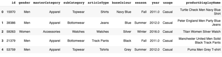
For this exercise we will classify fashion items into their sub category labels. To do this we extract the image ‘id’ column along with ‘subCategory’ to create a new labels file.

import pandas as pd
gt = pd.read_csv("./dataset/styles.csv",error_bad_lines=False)
label_gt = gt[['id','subCategory']]
label_gt['id'] = label_gt['id'].astype(str) + '.jpg'
label_gt.to_csv('./dataset/subCategory.csv',index=False)

Now that we have the images and label files ready, we can begin with creating experiments.

Monk with Pytorch

After importing MONK creating an experiment is simple. We can load Pytorch backend and create a new project and experiment.

import os
import sys
sys.path.append("./monk_v1/monk/");
import psutilfrom pytorch_prototype import prototype
ptf = prototype(verbose=1);
ptf.Prototype("fashion", "exp1");

Next we create the ‘Dataset’ object and setup the dataset and label path along with CNN architecture and number of epochs.(DOCS)

ptf.Default(dataset_path="./mod_dataset/images", 
             path_to_csv="./mod_dataset/subCategory.csv", 
             model_name="densenet121", 
             freeze_base_network=True, num_epochs=5);

We can check for missing or corrupt images and take a look at class imbalances using Monk’s EDA function (DOCS)

ptf.EDA(check_missing=True, check_corrupt=True);

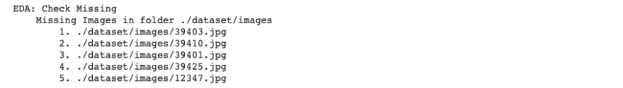Find missing images in your dataset

We have to update our labels file and remove rows containing missing or corrupt images. The notebook has a function ‘cleanCSV’ for this purpose.

After cleaning our labels file if we generated a new CSV, we have to update our ‘Dataset’ object to the location. This can be done by using the update functions (DOCS). Remember to run ‘Reload()’ after any making an update.

ptf.update_dataset(dataset_path="./dataset/images",
                   path_to_csv="./dataset/subCategory_cleaned.csv");
ptf.Reload()

And now we can start our training with:

ptf.Train()

For this experiment we are using densenet121 architecture. In the next experiments we will be using densenet169 and densenet201 architectures.

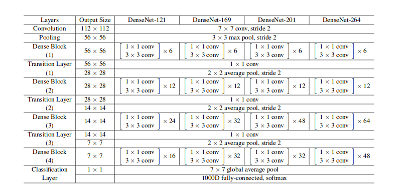Different Densenet architectures

After training is complete we get our final model accuracies and losses saved in our workspace folder. Now we can continue with the experiment and test our the other 2 densenet architectures.

ptf = prototype(verbose=1);
ptf.Prototype("fashion", "exp2");
ptf.Default(dataset_path="./dataset/images", 
            path_to_csv="./dataset/subCategory_cleaned.csv", 
            model_name="densenet169", freeze_base_network=True, 
            num_epochs=5);
ptf.Train()

AND

ptf = prototype(verbose=1);
ptf.Prototype("fashion", "exp3");
ptf.Default(dataset_path="./dataset/images", 
            path_to_csv="./dataset/subCategory_cleaned.csv", 
            model_name="densenet201", 
            freeze_base_network=True, num_epochs=5);
ptf.Train()

After training is complete for the 3 experiments we can quickly compare these and find out differences in losses(both training and validation), compare training time and resource utilisation and select the best model.

Since we have trained only for 5 epochs, it still will not be clear which architecture to choose from the 3, however, you can test out with either more epochs or even with a different CNN architecture. To update the model check out our DOCUMENTATION

Compare experiments

To run comparison we have to import the ‘compare’ module and add the 3 experiments.

from compare_prototype import compare
ctf = compare(verbose=1);
ctf.Comparison("Fashion_Pytorch_Densenet");
ctf.Add_Experiment("fashion", "exp1");
ctf.Add_Experiment("fashion", "exp2");
ctf.Add_Experiment("fashion", "exp3");

After adding the experiments to compare, we can generate the statistics. To find out more about the compare module check out (DOCS)

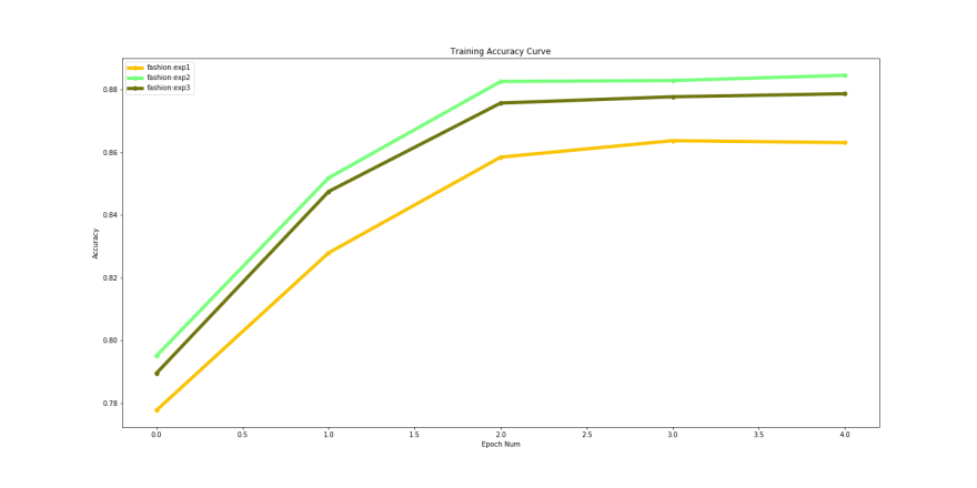Training accuracies over time

The training accuracy performance shows that ‘densenet169’ performs marginally better than the other 2. However looking at the validation accuracy shows us a different picture.

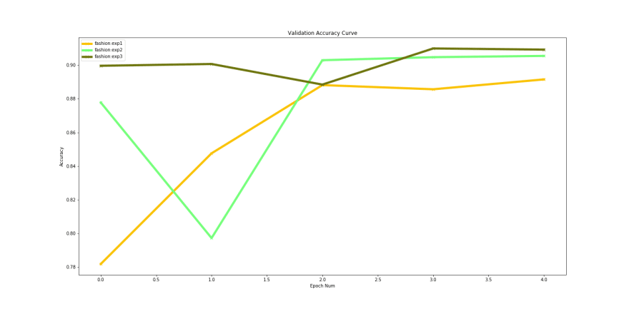Validation accuracies over time

Experiment 3 with ‘densenet201’ performs better that the others. If we compare the best validation accuracies for the 3 models, they are pretty close:

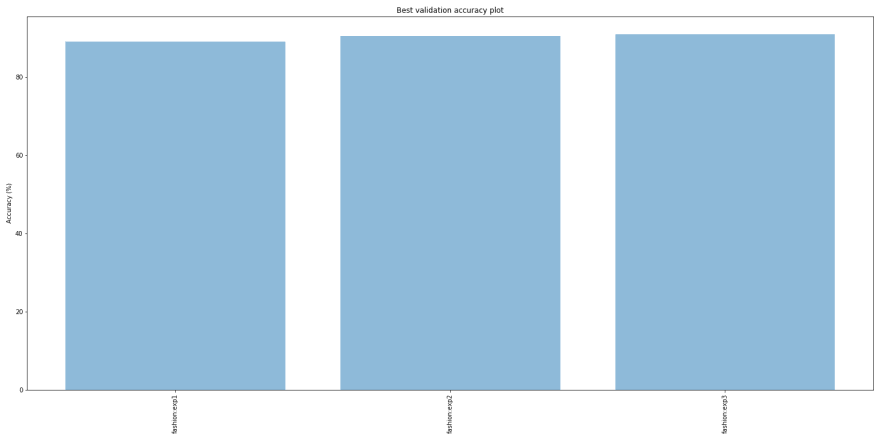Best validation accuracies

However one more metric to checkout before going ahead is the training times.

Training times

This shows that the more complex our CNN architecture the more time is takes to train per epoch.

Next we’ll create similar experiments but with Keras and Mxnet.

Monk with Mxnet

Monk is a syntax invariant library. So working with either of the available backend Deep Learning framework does not change the program you have to write.

The only change will be in import :

from gluon_prototype import prototype

Next we create experiments the same way with different densenet architectures and carry out training.

Gluon experiments —

gtf = prototype(verbose=1);
gtf.Prototype("fashion", "exp4");
gtf.Default(dataset_path="./dataset/images", 
            path_to_csv="./dataset/subCategory_cleaned.csv",
            model_name="densenet121", 
            freeze_base_network=True, num_epochs=5);
gtf.Train()

And so on…

Monk with Keras

As mentioned in the previous section, the only thing that changes is the import. So to utilise keras in the backend we import:

from keras_prototype import prototype

And then create some more experiments:

ktf = prototype(verbose=1);
ktf.Prototype("fashion", "exp7");
ktf.Default(dataset_path="./dataset/images", 
            path_to_csv="./dataset/subCategory_cleaned.csv", 
            model_name="densenet121", 
            freeze_base_network=True, num_epochs=5);
ktf.Train()

And so on…

Finally when we have trained the 9 experiments we can compare which framework and which architecture performed the best by using the compare utility in Monk(DOCS) and fine-tune the ones performing better.

Comparison plot for training accuracy generated from our exercise :

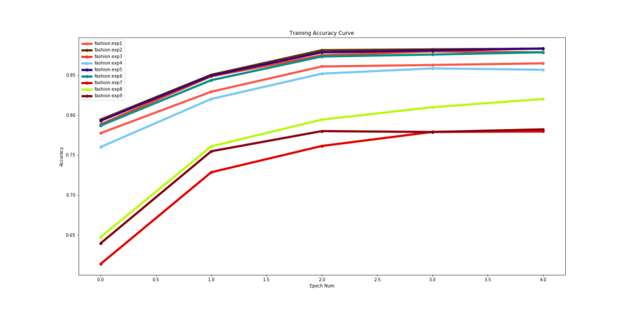Training accuracy comparisons

To achieve better results, try changing the learning rate schedulers and train for more epochs. You can easily copy an experiment and modify the hyper parameters, to generate better results. Check out our documentation for further instructions on this.

Happy Coding!