We are going to look at 4 different sorting algorithms and their implementation in Python:

• Bubble Sort
• Selection Sort
• Insertion Sort
• Quicksort

1. Bubble Sort

Time complexity: O(n²)

Implementation

def bubble(lst):
    no_swaps = False
    while no_swaps == False:
        no_swaps = True
        n = 0
        for i in range(len(lst) - 1 - n):
            if lst[i] > lst[i + 1]:
                lst[i], lst[i + 1] = lst[i + 1], lst[i]              
                no_swaps = False
        n += 1

How It Works

1. Iterate through the elements in the array
2. If there are adjacent elements in the wrong order, swap them
3. If we have reached the end of the array and there have been no swaps in this iteration, then the array is sorted. Else, repeat from step 1.

For example, suppose we have the following array:

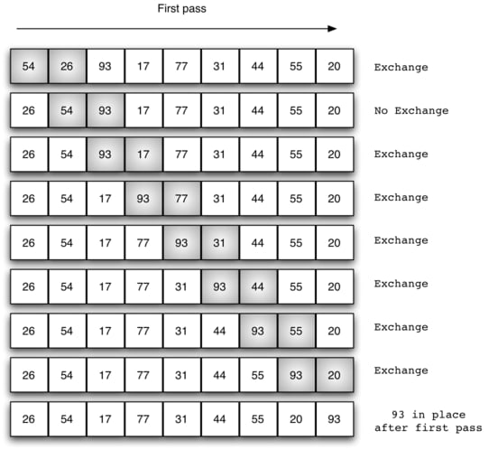
In the first pass, when i = 0, lst[0] = 54 and lst[1] = 26 . Since 26 < 54, and we want to sort the array in ascending order, we will swap the positions of 54 and 26 so that 26 comes before 54. This goes on until the end of the list.

Note that the largest element (93) always gets passed to the end of the array during the first iteration. This is the reason for the variable n which increases after each iteration and tells the program to exclude the last element after each iteration over the (sub)array.

The time complexity is O(n²) because it takes n iterations to guarantee a sorted array and every iteration iterates over n elements.

2. Selection Sort

Time complexity: O(n²)

Implementation

def selection(lst):
    for i in range(len(lst)):
        iMin = i
        for j in range(i + 1, len(lst)):
            if lst[j] < lst[iMin]:
                iMin = j
        lst[i], lst[iMin] = lst[iMin], lst[i]

How It Works

1. Iterate through the elements in the array
2. At each position, iterate through the unsorted elements to find the minimum element
3. Swap the positions of this minimum element and the element at the current position

For example, suppose we have the following array:

When i = 0, the minimum value within the unsorted array is 1, at position j = 3. Hence, the elements at position 0 and position 3 are swapped.

When i = 1, the minimum value within the unsorted array (the unsorted array is [5, 7, 8, 9, 3] since the first position is already sorted) is 3, at position j = 5. Hence, the elements in position 1 and 5 are swapped. The unsorted array is now [7, 8, 9, 5].

This goes on until the minimum value is selected (hence the name) for all positions. The time complexity is O(n²) since we have to iterate through the unsorted array n times, once for each current position, and the unsorted array consists of n elements on average.

3. Insertion Sort

Time complexity: O(n²)

Implementation

def insertion(lst):
    for i in range(1, len(lst)):
        temp = lst[i]
        j = i - 1
        while j >= 0 and temp < lst[j]:
            lst[j + 1] = lst[j]
            j -= 1
        lst[j + 1] = temp

How It Works

1. Iterate through the elements in the array

2. For each element, iterate through the sorted array to find a suitable position (where it is larger than the element right before it, and smaller than the element right after it)

   For example, when i = 5 and lst[i] = 31, I want to insert (hence the name) 31 into the sorted array. The while loop will ‘copy’ the element at j to the position j + 1 and decrease the value of j, until 31 > lst[j]. This occurs at j = 1, where lst[j] = 26. Since 26 < 31 < 54, the right position to insert 31 would be at j + 1 = 2.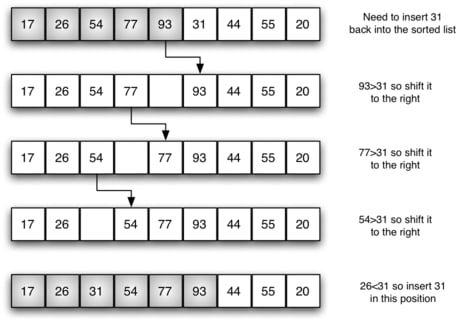

   

3. Insert the element at its suitable position. From step 2, all the elements from this position onwards are ‘pushed back’ to the right by one position to make space for the inserted element

For example, suppose we have the following array:

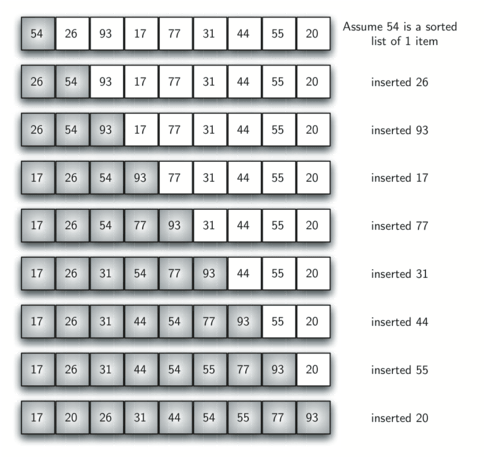
When i = 0, there is no sorted array and we simply move on to i = 1. Note that this case is captured under one of the while loop exit conditions; since j >= 0 is False, the while loop will not be run.

When i = 1, the sorted array consists of [54,], and the current element is 26. The correct position to insert 26 is before 54, so 54 is ‘pushed back’ to the right (it is now at position 1) and 26 is inserted at position 0.

This goes on until all the elements are inserted at their suitable positions and the whole array is sorted. The time complexity is O(n²) because we have to iterate through the sorted list n times to find a suitable position for all n elements, and the sorted list consists of n elements on average.

4. Quicksort

Time complexity: O(n log(n))

Implementation (out-of-place)

def quicksort(lst):

    if len(lst) == 0:
        return lst

    else:
        pivot = lst[0]
        left = []
        right = []

        for ele in lst:

            if ele < pivot:
                left.append(ele)

            if ele > pivot:
                right.append(ele)

        return quicksort(left) + [pivot] + quicksort(right)

Implementation (in-place)

def partition(lst, start, end):

    # partition list into left (< pivot), middle (pivot) and right (> pivot), and return position of pivot

    pivot = lst[start]
    left = start + 1
    right = end

    done = False    
    while not done:        

        # find left position where element > pivot
        while left <= right and lst[left] < pivot:
            left += 1        

        # find right position where element < pivot
        while right >= left and lst[right] > pivot:
            right -= 1

        if left > right:
            # stop sorting
            done = True

        else:
            # lst[left] now < pivot, lst[right] now > pivot            
            lst[left], lst[right] = lst[right], lst[left]

    # place pivot in the correct position
    lst[start], lst[right] = lst[right], lst[start]

    return right        

def quicksort_in_place(lst, start, end):

    # sort list recursively with the help of partition()

    if start < end:

        pivot = partition(lst, start, end)    

        quicksort_in_place(lst, start, pivot - 1)        
        quicksort_in_place(lst, pivot + 1, end)

How It Works

This is a recursive algorithm. For each recursive call,

1. The first element of the array is taken as the ‘pivot’
2. Partition the array so that you have a subarray of elements that are smaller than the pivot, and another subarray of elements that are larger than the pivot. Position the pivot in the middle of the two subarrays.
3. Recursively sort both subarrays

The base case: when the subarray is empty (or contains only one element), it cannot be sorted any further.

The In-Place Algorithm

The in-place algorithm modifies the original array, whereas the out-of-place algorithm creates and returns a new array that is a sorted version of the original array. The recursion logic is pretty much the same, except the partition() function can be a bit confusing.

The partition function involves left and right pointers. The left pointer moves to the right until it finds an element that is larger than the pivot. The right pointer moves to the left until it finds an element that is smaller than the pivot. These two elements are then swapped because we want everything on the left to be smaller than the pivot, and everything on the right to be larger than the pivot.

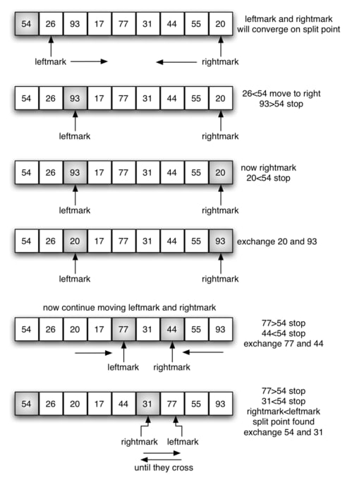
This continues until the left and right pointers cross positions. At this point, we have (almost) successfully partitioned the array. Everything before the left pointer is smaller than the pivot, and everything after the right pointer is larger than the pivot. The last step involves exchanging the positions of the pivot and the element at the right pointer so that the pivot now lies between the left and right subarrays.

The left subarray consists of everything before the pivot, and everything in this subarray is smaller than the pivot. The right subarray consists of everything after the pivot, and everything in this subarray is larger than the pivot.

We have now successfully partitioned the array. This process is repeated on each subarray until the entire array is sorted.

Time Complexity

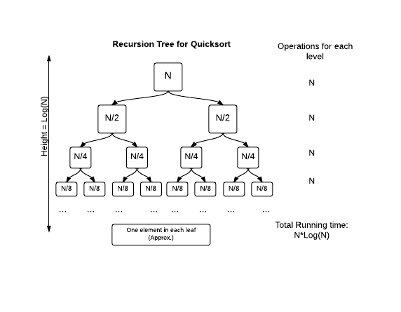
Working from the bottom-up, 1×2ʰ = n where h is the height of the recursive tree and n is the size of the array. This is because starting from a ‘leaf’ (a one-element subarray), every layer above it merges two subarrays to form a new array that is twice the length of each individual subarray. The size of the subarray, therefore, roughly doubles every time it goes ‘up’ a layer. Therefore, h, the height of the recursive tree, is log(n).

At each layer of the recursive tree, a total of n comparisons are made to partition each subarray (since the total number of elements is still n).

Hence, the overall time complexity is O(n log(n)).

Conclusion

Thanks for reading! If you have any questions, feel free to comment on this post.

Follow me for more stories like this one in the future.