
Author: Jacob Marks (Machine Learning Engineer at Voxel51)
Run and Evaluate Monocular Depth Estimation Models with Hugging Face and FiftyOne
Humans view the world through two eyes. One of the primary benefits of this binocular vision is the ability to perceive depth — how near or far objects are. The human brain infers object depths by comparing the pictures captured by left and right eyes at the same time and interpreting the disparities. This process is known as stereopsis.
Just as depth perception plays a crucial role in human vision and navigation, the ability to estimate depth is critical for a wide range of computer vision applications, from autonomous driving to robotics, and even augmented reality. Yet a slew of practical considerations from spatial limitations to budgetary constraints often limit these applications to a single camera.
Monocular depth estimation (MDE) is the task of predicting the depth of a scene from a single image. Depth computation from a single image is inherently ambiguous, as there are multiple ways to project the same 3D scene onto the 2D plane of an image. As a result, MDE is a challenging task that requires (either explicitly or implicitly) factoring in many cues such as object size, occlusion, and perspective.
In this post, we will illustrate how to load and visualize depth map data, run monocular depth estimation models, and evaluate depth predictions. We will do so using data from the SUN-RGBD dataset.
In particular, we will cover the following:
- Loading and visualizing SUN-RGBD ground truth depth maps
- Running inference with Marigold and DPT
- Evaluating relative depth predictions
We will use the Hugging Face transformers and diffusers libraries for inference, FiftyOne for data management and visualization, and scikit-image for evaluation metrics.
Before we get started, make sure you have all of the necessary libraries installed:
pip install -U torch fiftyone diffusers transformers scikit-image
Then we’ll import the modules we’ll be using throughout the post:
from glob import glob
import numpy as np
from PIL import Image
import torch

import fiftyone as fo
import fiftyone.zoo as foz
import fiftyone.brain as fob
from fiftyone import ViewField as F
Loading and Visualizing SUN-RGBD Depth Data
The SUN RGB-D dataset contains 10,335 RGB-D images, each of which has a corresponding RGB image, depth image, and camera intrinsics. It contains images from the NYU depth v2, Berkeley B3DO, and SUN3D datasets. SUN RGB-D is one of the most popular datasets for monocular depth estimation and semantic segmentation tasks!
💡For this walkthrough, we will only use the NYU depth v2 portions. NYU depth v2 is permissively licensed for commercial use (MIT), and can be downloaded from Hugging Face directly.
Downloading the Raw Data
First, download the SUN RGB-D dataset from here and unzip it, or use the following command to download it directly:
curl -o sunrgbd.zip https://rgbd.cs.princeton.edu/data/SUNRGBD.zip
And then unzip it:
unzip sunrgbd.zip
If you want to use the dataset for other tasks, you can fully convert the annotations and load them into your fiftyone.Dataset. However, for this tutorial, we will only be using the depth images, so we will only use the RGB images and the depth images (stored in the depth_bfx sub-directories).
Creating the Dataset
Because we are just interested in getting the point across, we'll restrict ourselves to the first 20 samples, which are all from the NYU Depth v2 portion of the dataset:
## create, name, and persist the dataset
dataset = fo.Dataset(name="SUNRGBD-20", persistent=True)

## pick out first 20 scenes
scene_dirs = glob("SUNRGBD/kv1/NYUdata/*")[:20]

samples = []

for scene_dir in scene_dirs:
    ## Get image file path from scene directory
    image_path = glob(f"{scene_dir}/image/*")[0]

    ## Get depth map file path from scene directory
    depth_path = glob(f"{scene_dir}/depth_bfx/*")[0]

    depth_map = np.array(Image.open(depth_path))
    depth_map = (depth_map * 255 / np.max(depth_map)).astype("uint8")

    ## Create sample
    sample = fo.Sample(
        filepath=image_path,
        gt_depth=fo.Heatmap(map=depth_map),
    )

    samples.append(sample)

## Add samples to dataset
dataset.add_samples(samples);
Here we are storing the depth maps as heatmaps. Everything is represented in terms of normalized, relative distances, where 255 represents the maximum distance in the scene and 0 represents the minimum distance in the scene. This is a common way to represent depth maps, although it is far from the only way to do so. If we were interested in absolute distances, we could store sample-wise parameters for the minimum and maximum distances in the scene, and use these to reconstruct the absolute distances from the relative distances.
Visualizing Ground Truth Data
With heatmaps stored on our samples, we can visualize the ground truth data:
session = fo.launch_app(dataset, auto=False)
## then open tab to localhost:5151 in browser
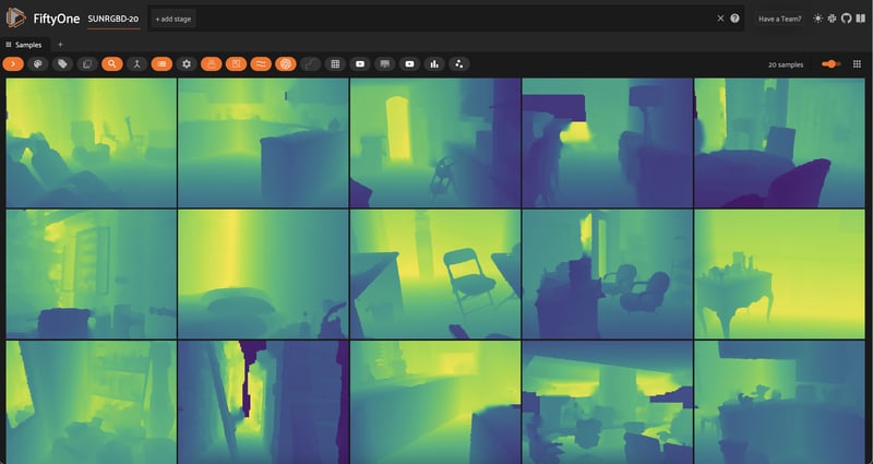
When working with depth maps, the color scheme and opacity of the heatmap are important. I’m colorblind, so I find that the viridis colormap with opacity turned all the way up works best for me.

Ground Truth?
Inspecting these RGB images and depth maps, we can see that there are some inaccuracies in the ground truth depth maps. For example, in this image, the dark rift through the center of the image is actually the farthest part of the scene, but the ground truth depth map shows it as the closest part of the scene:

This is one of the key challenges for MDE tasks: ground truth data is hard to come by, and is often noisy! It’s essential to be aware of this while evaluating your MDE models.
Running Monocular Depth Estimation Models
Now that we have our dataset loaded in, we can run monocular depth estimation models on our RGB images!
For a long time, the state-of-the-art models for monocular depth estimation such as DORN and DenseDepth were built with convolutional neural networks. Recently, however, both transformer-based models such as DPT and GLPN, and diffusion-based models like Marigold have achieved remarkable results!
In this section, we’ll show you how to generate MDE depth map predictions with both DPT and Marigold. In both cases, you can optionally run the model locally with the respective Hugging Face library, or run remotely with Replicate.
To run via Replicate, install the Python client:
pip install replicate
And export your Replicate API token:
export REPLICATE_API_TOKEN=r8_<your_token_here>
💡 With Replicate, it might take a minute for the model to load into memory on the server (cold-start problem), but once it does the prediction should only take a few seconds. Depending on your local compute resources, running on server may give you massive speedups compared to running locally, especially for Marigold and other diffusion-based depth-estimation approaches.
Monocular Depth Estimation with DPT
The first model we will run is a dense-prediction transformer (DPT). DPT models have found utility in both MDE and semantic segmentation — tasks that require “dense”, pixel-level predictions.
The checkpoint below uses MiDaS, which returns the inverse depth map, so we have to invert it back to get a comparable depth map.
To run locally with transformers, first we load the model and image processor:
from transformers import AutoImageProcessor, AutoModelForDepthEstimation

## swap for "Intel/dpt-large" if you'd like
pretrained = "Intel/dpt-hybrid-midas"

image_processor = AutoImageProcessor.from_pretrained(pretrained)
dpt_model = AutoModelForDepthEstimation.from_pretrained(pretrained)
Next, we encapsulate the code for inference on a sample, including pre and post processing:
def apply_dpt_model(sample, model, label_field):
    image = Image.open(sample.filepath)
    inputs = image_processor(images=image, return_tensors="pt")

    with torch.no_grad():
        outputs = model(**inputs)
        predicted_depth = outputs.predicted_depth

    prediction = torch.nn.functional.interpolate(
        predicted_depth.unsqueeze(1),
        size=image.size[::-1],
        mode="bicubic",
        align_corners=False,
    )

    output = prediction.squeeze().cpu().numpy()
    ## flip b/c MiDaS returns inverse depth
    formatted = (255 - output * 255 / np.max(output)).astype("uint8")

    sample[label_field] = fo.Heatmap(map=formatted)
    sample.save()
Here, we are storing predictions in a label_field field on our samples, represented with a heatmap just like the ground truth labels.
Note that in the apply_dpt_model() function, between the model's forward pass and the heatmap generation, notice that we make a call to torch.nn.functional.interpolate(). This is because the model's forward pass is run on a downsampled version of the image, and we want to return a heatmap that is the same size as the original image.
Why do we need to do this? If we just want to look at the heatmaps, this would not matter. But if we want to compare the ground truth depth maps to the model's predictions on a per-pixel basis, we need to make sure that they are the same size.
All that is left to do is iterate through the dataset:
for sample in dataset.iter_samples(autosave=True, progress=True):
    apply_dpt_model(sample, dpt_model, "dpt")

session = fo.launch_app(dataset)

To run with Replicate, you can use this model. Here is what the API looks like:
import replicate

## example application to first sample
rgb_fp = dataset.first().filepath

output = replicate.run(
    "cjwbw/midas:a6ba5798f04f80d3b314de0f0a62277f21ab3503c60c84d4817de83c5edfdae0",
    input={
        "model_type": "dpt_beit_large_512",
        "image":open(rgb_fp, "rb")
    }
)
print(output)
Monocular Depth Estimation with Marigold
Stemming from their tremendous success in text-to-image contexts, diffusion models are being applied to an ever-broadening range of problems. Marigold “repurposes” diffusion-based image generation models for monocular depth estimation.
To run Marigold locally, you will need to clone the git repository:
git clone https://github.com/prs-eth/Marigold.git
This repository introduces a new diffusers pipeline, MarigoldPipeline, which makes applying Marigold easy:
## load model
from Marigold.marigold import MarigoldPipeline
pipe = MarigoldPipeline.from_pretrained("Bingxin/Marigold")

## apply to first sample, as example
rgb_image = Image.open(dataset.first().filepath)
output = pipe(rgb_image)
depth_image = output['depth_colored']
Post-processing of the output depth image is then needed.
To instead run via Replicate, we can create an apply_marigold_model() function in analogy with the DPT case above and iterate over the samples in our dataset:
import replicate
import requests
import io

def marigold_model(rgb_image):
    output = replicate.run(
        "adirik/marigold:1a363593bc4882684fc58042d19db5e13a810e44e02f8d4c32afd1eb30464818",
        input={
            "image":rgb_image
        }
    )
    ## get the black and white depth map
    response = requests.get(output[1]).content
    return response

def apply_marigold_model(sample, model, label_field):
    rgb_image = open(sample.filepath, "rb")
    response = model(rgb_image)
    depth_image = np.array(Image.open(io.BytesIO(response)))[:, :, 0] ## all channels are the same
    formatted = (255 - depth_image).astype("uint8")
    sample[label_field] = fo.Heatmap(map=formatted)
    sample.save()

for sample in dataset.iter_samples(autosave=True, progress=True):
    apply_marigold_model(sample, marigold_model, "marigold")

session = fo.launch_app(dataset)

Evaluating Monocular Depth Estimation Models
Now that we have predictions from multiple models, let's evaluate them! We will leverage scikit-image to apply three simple metrics commonly used for monocular depth estimation: root mean squared error (RMSE), peak signal to noise ratio (PSNR), and structural similarity index (SSIM).
💡Higher PSNR and SSIM scores indicate better predictions, while lower RMSE scores indicate better predictions.
Note that the specific values I arrive at are a consequence of the specific pre-and-post processing steps I performed along the way. What matters is the relative performance!
We will define the evaluation routine:
from skimage.metrics import peak_signal_noise_ratio, mean_squared_error, structural_similarity

def rmse(gt, pred):
    """Compute root mean squared error between ground truth and prediction"""
    return np.sqrt(mean_squared_error(gt, pred))

def evaluate_depth(dataset, prediction_field, gt_field):
  """Run 3 evaluation metrics for all samples for `prediction_field`
     with respect to `gt_field`"""
    for sample in dataset.iter_samples(autosave=True, progress=True):
        gt_map = sample[gt_field].map
        pred = sample[prediction_field]
        pred_map = pred.map
        pred["rmse"] = rmse(gt_map, pred_map)
        pred["psnr"] = peak_signal_noise_ratio(gt_map, pred_map)
        pred["ssim"] = structural_similarity(gt_map, pred_map)
        sample[prediction_field] = pred

    ## add dynamic fields to dataset so we can view them in the App
    dataset.add_dynamic_sample_fields()
And then apply the evaluation to the predictions from both models:
evaluate_depth(dataset, "dpt", "gt_depth")
evaluate_depth(dataset, "marigold", "gt_depth")
Computing average performance for a certain model/metric is as simple as calling the dataset’s mean()method on that field:
print("Mean Error Metrics")
for model in ["dpt", "marigold"]:
    print("-"*50)
    for metric in ["rmse", "psnr", "ssim"]:
        mean_metric_value = dataset.mean(f"{model}.{metric}")
        print(f"Mean {metric} for {model}: {mean_metric_value}")
Mean Error Metrics
--------------------------------------------------
Mean rmse for dpt: 49.8915828817003
Mean psnr for dpt: 14.805904629602551
Mean ssim for dpt: 0.8398022368184576
--------------------------------------------------
Mean rmse for marigold: 104.0061165272178
Mean psnr for marigold: 7.93015537185192
Mean ssim for marigold: 0.42766803372861134
All of the metrics seem to agree that DPT outperforms Marigold. However, it is important to note that these metrics are not perfect. For example, RMSE is very sensitive to outliers, and SSIM is not very sensitive to small errors. For a more thorough evaluation, we can filter by these metrics in the app in order to visualize what the model is doing well and what it is doing poorly — or where the metrics are failing to capture the model's performance.
Finally, toggling masks on and off is a great way to visualize the differences between the ground truth and the model's predictions:

Conclusion
To recap, we learned how to run monocular depth estimation models on our data, how to evaluate the predictions using common metrics, and how to visualize the results. We also learned that monocular depth estimation is a notoriously difficult task.
Data quality and quantity are severely limiting factors; models often struggle to generalize to new environments; and metrics are not always good indicators of model performance. The specific numeric values quantifying model performance can depend greatly on your processing pipeline. And even your qualitative assessment of predicted depth maps can be heavily influenced by your color schemes and opacity scales.
If there’s one thing you take away from this post, I hope it is this: it is mission-critical that you look at the depth maps themselves, and not just the metrics!


Top comments (0)