
Just like writing your very first for loop, understanding time complexity is an integral milestone to learning how to write efficient complex programs. Think of it as having a superpower that allows you to know exactly what type of program might be the most efficient in a particular situation - before even running a single line of code.
The fundamental concepts of complexity analysis are well worth studying. You'll be able to better understand how the code you're writing will interact with the program's input, and as a result, you'll spend a lot less wasted time writing slow and problematic code. It won't take long to go over all you need to know in order to start writing more efficient programs - in fact, we can do it in about fifteen minutes. You can go grab a coffee right now (or tea, if that's your thing) and I'll take you through it before your coffee break is over. Go ahead, I'll wait.
All set? Let's do it!
What is "time complexity" anyway?
The time complexity of an algorithm is an approximation of how long that algorithm will take to process some input. It describes the efficiency of the algorithm by the magnitude of its operations. This is different than the number of times an operation repeats; I'll expand on that later. Generally, the fewer operations the algorithm has, the faster it will be.
We write about time complexity using Big O notation, which looks something like O(n). There's rather a lot of math involved in its formal definition, but informally we can say that Big O notation gives us our algorithm's approximate run time in the worst case, or in other words, its upper bound.[2] It is inherently relative and comparative.[3] We're describing the algorithm's efficiency relative to the increasing size of its input data, n. If the input is a string, then n is the length of the string. If it's a list of integers, n is the length of the list.
It's easiest to picture what Big O notation represents with a graph:
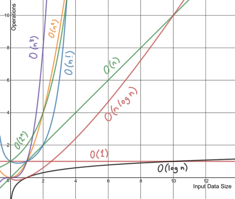
Lines made with the very excellent Desmos graph calculator. You can play with this graph here.
Here are the main important points to remember as you read the rest of this article:
- Time complexity is an approximation
- An algorithm's time complexity approximates its worst case run time
Determining time complexity
There are different classes of complexity that we can use to quickly understand an algorithm. I'll illustrate some of these classes using nested loops and other examples.
Polynomial time complexity
A polynomial, from the Greek poly meaning "many," and Latin nomen meaning "name," describes an expression comprised of constant variables, and addition, multiplication, and exponentiation to a non-negative integer power.[4] That's a super math-y way to say that it contains variables usually denoted by letters, and symbols that look like these:

The below classes describe polynomial algorithms. Some have food examples.
Constant
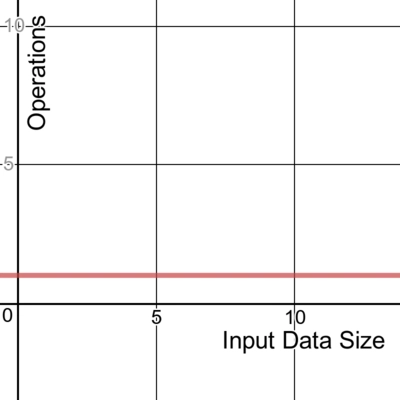
A constant time algorithm doesn't change its running time in response to the input data. No matter the size of the data it receives, the algorithm takes the same amount of time to run. We denote this as a time complexity of O(1).
Here's one example of a constant algorithm that takes the first item in a slice.
func takeCupcake(cupcakes []int) int {
    return cupcakes[0]
}

Choice of flavours are: vanilla cupcake, strawberry cupcake, mint chocolate cupcake, lemon cupcake, and "wibbly wobbly, timey wimey" cupcake.
With this contant-time algorithm, no matter how many cupcakes are on offer, you just get the first one. Oh well. Flavours are overrated anyway.
Linear
The running duration of a linear algorithm is constant. It will process the input in n number of operations. This is often the best possible (most efficient) case for time complexity where all the data must be examined.

Here's an example of code with time complexity of O(n):
func eatChips(bowlOfChips int) {
    for chip := 0; chip <= bowlOfChips; chip++ {
        // dip chip
    }
}
Here's another example of code with time complexity of O(n):
func eatChips(bowlOfChips int) {
    for chip := 0; chip <= bowlOfChips; chip++ {
        // double dip chip
    }
}
It doesn't matter whether the code inside the loop executes once, twice, or any number of times. Both these loops process the input by a constant factor of n, and thus can be described as linear.

Don't double dip in a shared bowl.
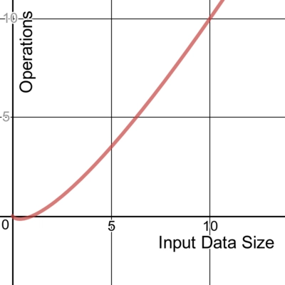
Quadratic

Now here's an example of code with time complexity of O(n2):
func pizzaDelivery(pizzas int) {
    for pizza := 0; pizza <= pizzas; pizza++ {
        // slice pizza
        for slice := 0; slice <= pizza; slice++ {
            // eat slice of pizza
        }
    }
}
Because there are two nested loops, or nested linear operations, the algorithm process the input n2 times.
Cubic
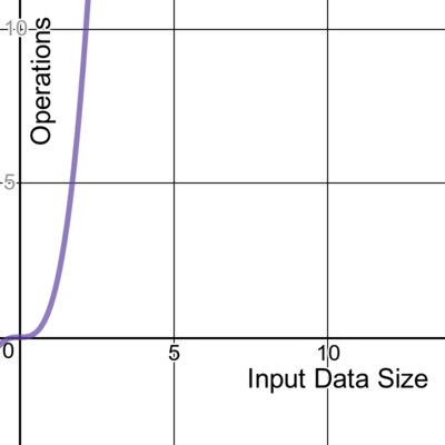
Extending on the previous example, this code with three nested loops has time complexity of O(n3):
func pizzaDelivery(boxesDelivered int) {
    for pizzaBox := 0; pizzaBox <= boxesDelivered; pizzaBox++ {
        // open box
        for pizza := 0; pizza <= pizzaBox; pizza++ {
            // slice pizza
            for slice := 0; slice <= pizza; slice++ {
                // eat slice of pizza
            }
        }
    }
}

Seriously though, who delivers unsliced pizza??
Logarithmic
A logarithmic algorithm is one that reduces the size of the input at every step.
We denote this time complexity as O(log n), where log, the logarithm function, is this shape:

One example of this is a binary search algorithm that finds the position of an element within a sorted array. Here's how it would work, assuming we're trying to find the element x:
- If x matches the middle element m of the array, return the position of m
- If x doesn't match m, see if m is larger or smaller than x
- If larger, discard all array items greater than m
- If smaller, discard all array items smaller than m
- Continue by repeating steps 1 and 2 on the remaining array until x is found
I find the clearest analogy for understanding binary search is imagining the process of locating a book in a bookstore aisle. If the books are organized by author's last name and you want to find "Terry Pratchett," you know you need to look for the "P" section.
You can approach the shelf at any point along the aisle and look at the author's last name there. If you're looking at a book by Neil Gaiman, you know you can ignore all the rest of the books to your left, since no letters that come before "G" in the alphabet happen to be "P." You would then move down the aisle to the right any amount, and repeat this process until you've found the Terry Pratchett section, which should be rather sizable if you're at any decent bookstore because wow did he write a lot of books.
Quasilinear
Often seen with sorting algorithms, the time complexity O(n log n) can describe a data structure where each operation takes O(log n) time. One example of this is quick sort, a divide-and-conquer algorithm.
Quick sort works by dividing up an unsorted array into smaller chunks that are easier to process. It sorts the sub-arrays, and thus the whole array. Think about it like trying to put a deck of cards in order. It's faster if you split up the cards and get five friends to help you.
Non-polynomial time complexity
The below classes of algorithms are non-polynomial.
Factorial

An algorithm with time complexity O(n!) often iterates through all permutations of the input elements. One common example is a brute-force search seen in the travelling salesman problem. It tries to find the least costly path between a number of points by enumerating all possible permutations and finding the ones with the lowest cost.
Exponential
An exponential algorithm often also iterates through all subsets of the input elements. It is denoted O(2n) and is often seen in brute-force algorithms. It is similar to factorial time except in its rate of growth, which as you may not be surprised to hear, is exponential. The larger the data set, the more steep the curve becomes.

In cryptography, a brute-force attack may systematically check all possible elements of a password by iterating through subsets. Using an exponential algorithm to do this, it becomes incredibly resource-expensive to brute-force crack a long password versus a shorter one. This is one reason that a long password is considered more secure than a shorter one.
There are further time complexity classes less commonly seen that I won't cover here, but you can read about these and find examples in this handy table.
Recursion time complexity
As I described in my article explaining recursion using apple pie, a recursive function calls itself under specified conditions. Its time complexity depends on how many times the function is called and the time complexity of a single function call. In other words, it's the product of the number of times the function runs and a single execution's time complexity.
Here's a recursive function that eats pies until no pies are left:
func eatPies(pies int) int {
    if pies == 0 {
        return pies
    }
    return eatPies(pies - 1)
}
The time complexity of a single execution is constant. No matter how many pies are input, the program will do the same thing: check to see if the input is 0. If so, return, and if not, call itself with one fewer pie.
The initial number of pies could be any number, and we need to process all of them, so we can describe the input as n. Thus, the time complexity of this recursive function is the product O(n).

This function's return value is zero, plus some indigestion.
Worst case time complexity
So far, we've talked about the time complexity of a few nested loops and some code examples. Most algorithms, however, are built from many combinations of these. How do we determine the time complexity of an algorithm containing many of these elements strung together?
Easy. We can describe the total time complexity of the algorithm by finding the largest complexity among all of its parts. This is because the slowest part of the code is the bottleneck, and time complexity is concerned with describing the worst case for the algorithm's run time.
Say we have a program for an office party. If our program looks like this:
package main

import "fmt"

func takeCupcake(cupcakes []int) int {
    fmt.Println("Have cupcake number",cupcakes[0])
    return cupcakes[0]
}

func eatChips(bowlOfChips int) {
    fmt.Println("Have some chips!")
    for chip := 0; chip <= bowlOfChips; chip++ {
        // dip chip
    }
    fmt.Println("No more chips.")
}

func pizzaDelivery(boxesDelivered int) {
    fmt.Println("Pizza is here!")
    for pizzaBox := 0; pizzaBox <= boxesDelivered; pizzaBox++ {
        // open box
        for pizza := 0; pizza <= pizzaBox; pizza++ {
            // slice pizza
            for slice := 0; slice <= pizza; slice++ {
                // eat slice of pizza
            }
        }
    }
    fmt.Println("Pizza is gone.")
}

func eatPies(pies int) int {
    if pies == 0 {
        fmt.Println("Someone ate all the pies!")
        return pies
    }
    fmt.Println("Eating pie...")
    return eatPies(pies - 1)
}

func main() {
    takeCupcake([]int{1, 2, 3})
    eatChips(23)
    pizzaDelivery(3)
    eatPies(3)
    fmt.Println("Food gone. Back to work!")
}
We can describe the time complexity of all the code by the complexity of its most complex part. This program is made up of functions we've already seen, with the following time complexity classes:
| Function | Class | Big O |
|---|---|---|
takeCupcake |
constant | O(1) |
eatChips |
linear | O(n) |
pizzaDelivery |
cubic | O(n3) |
eatPies |
linear (recursive) | O(n) |
To describe the time complexity of the entire office party program, we choose the worst case. This program would have the time complexity O(n3).
Here's the office party soundtrack, just for fun.
Have cupcake number 1
Have some chips!
No more chips.
Pizza is here!
Pizza is gone.
Eating pie...
Eating pie...
Eating pie...
Someone ate all the pies!
Food gone. Back to work!
P vs NP, NP-complete, and NP-hard
You may come across these terms in your explorations of time complexity. Informally, P (for Polynomial time), is a class of problems that is quick to solve. NP, for Nondeterministic Polynomial time, is a class of problems where the answer can be quickly verified in polynomial time. NP encompasses P, but also another class of problems called NP-complete, for which no fast solution is known.[5] Outside of NP but still including NP-complete is yet another class called NP-hard, which includes problems that no one has been able to verifiably solve with polynomial algorithms.[6]

P vs NP Euler diagram, by Behnam Esfahbod, CC BY-SA 3.0
P versus NP is an unsolved, open question in computer science.
Anyway, you don't generally need to know about NP and NP-hard problems to begin taking advantage of understanding time complexity. They're a whole other Pandora's box.
Approximate the efficiency of an algorithm before you write the code
So far, we've identified some different time complexity classes and how we might determine which one an algorithm falls into. So how does this help us before we've written any code to evaluate?
By combining a little knowledge of time complexity with an awareness of the size of our input data, we can take a guess at an efficient algorithm for processing our data within a given time constraint. We can base our estimation on the fact that a modern computer can perform some hundreds of millions of operations in a second.[1] The following table from the Competitive Programmer's Handbook offers some estimates on required time complexity to process the respective input size in a time limit of one second.
| Input size | Required time complexity for 1s processing time |
|---|---|
| n ≤ 10 | O(n!) |
| n ≤ 20 | O(2n) |
| n ≤ 500 | O(n3) |
| n ≤ 5000 | O(n2) |
| n ≤ 106 | O(n log n) or O(n) |
| n is large | O(1) or O(log n) |
Keep in mind that time complexity is an approximation, and not a guarantee. We can save a lot of time and effort by immediately ruling out algorithm designs that are unlikely to suit our constraints, but we must also consider that Big O notation doesn't account for constant factors. Here's some code to illustrate.
The following two algorithms both have O(n) time complexity.
func makeCoffee(scoops int) {
    for scoop := 0; scoop <= scoops; scoop++ {
        // add instant coffee
    }
}
func makeStrongCoffee(scoops int) {
    for scoop := 0; scoop <= 3*scoops; scoop++ {
        // add instant coffee
    }
}
The first function makes a cup of coffee with the number of scoops we ask for. The second function also makes a cup of coffee, but it triples the number of scoops we ask for. To see an illustrative example, let's ask both these functions for a cup of coffee with a million scoops.
Here's the output of the Go test:
Benchmark_makeCoffee-4          1000000000               0.29 ns/op
Benchmark_makeStrongCoffee-4    1000000000               0.86 ns/op
Our first function, makeCoffee, completed in an average 0.29 nanoseconds. Our second function, makeStrongCoffee, completed in an average of 0.86 nanoseconds. While those may both seem like pretty small numbers, consider that the stronger coffee took near three times longer to make. This should make sense intuitively, since we asked it to triple the scoops. Big O notation alone wouldn't tell you this, since the constant factor of the tripled scoops isn't accounted for.
Improve time complexity of existing code
Becoming familiar with time complexity gives us the opportunity to write code, or refactor code, to be more efficient. To illustrate, I'll give a concrete example of one way we can refactor a bit of code to improve its time complexity.
Let's say a bunch of people at the office want some pie. Some people want pie more than others. The amount that everyone wants some pie is represented by an int > 0:
diners := []int{2, 88, 87, 16, 42, 10, 34, 1, 43, 56}
Unfortunately, we're bootstrapped and there are only three forks to go around. Since we're a cooperative bunch, the three people who want pie the most will receive the forks to eat it with. Even though they've all agreed on this, no one seems to want to sort themselves out and line up in an orderly fashion, so we'll have to make do with everybody jumbled about.
Without sorting the list of diners, return the three largest integers in the slice.
Here's a function that solves this problem and has O(n2) time complexity:
func giveForks(diners []int) []int {
    // make a slice to store diners who will receive forks
    var withForks []int
    // loop over three forks
    for i := 1; i <= 3; i++ {
        // variables to keep track of the highest integer and where it is
        var max, maxIndex int
        // loop over the diners slice
        for n := range diners {
            // if this integer is higher than max, update max and maxIndex
            if diners[n] > max {
                max = diners[n]
                maxIndex = n
            }
        }
        // remove the highest integer from the diners slice for the next loop
        diners = append(diners[:maxIndex], diners[maxIndex+1:]...)
        // keep track of who gets a fork
        withForks = append(withForks, max)
    }
    return withForks
}
This program works, and eventually returns diners [88 87 56]. Everyone gets a little impatient while it's running though, since it takes rather a long time (about 120 nanoseconds) just to hand out three forks, and the pie's getting cold. How could we improve it?
By thinking about our approach in a slightly different way, we can refactor this program to have O(n) time complexity:
func giveForks(diners []int) []int {
    // make a slice to store diners who will receive forks
    var withForks []int
    // create variables for each fork
    var first, second, third int
    // loop over the diners
    for i := range diners {
        // assign the forks
        if diners[i] > first {
            third = second
            second = first
            first = diners[i]
        } else if diners[i] > second {
            third = second
            second = diners[i]
        } else if diners[i] > third {
            third = diners[i]
        }
    }
    // list the final result of who gets a fork
    withForks = append(withForks, first, second, third)
    return withForks
}
Here's how the new program works:
Initially, diner 2 (the first in the list) is assigned the first fork. The other forks remain unassigned.
Then, diner 88 is assigned the first fork instead. Diner 2 gets the second one.
Diner 87 isn't greater than first which is currently 88, but it is greater than 2 who has the second fork. So, the second fork goes to 87. Diner 2 gets the third fork.
Continuing in this violent and rapid fork exchange, diner 16 is then assigned the third fork instead of 2, and so on.
We can add a print statement in the loop to see how the fork assignments play out:
0 0 0
2 0 0
88 2 0
88 87 2
88 87 16
88 87 42
88 87 42
88 87 42
88 87 42
88 87 43
[88 87 56]
This program is much faster, and the whole epic struggle for fork domination is over in 47 nanoseconds.
As you can see, with a little change in perspective and some refactoring, we've made this simple bit of code faster and more efficient.
Well, it looks like our fifteen minute coffee break is up! I hope I've given you a comprehensive introduction to calculating time complexity. Time to get back to work, hopefully applying your new knowledge to write more effective code! Or maybe just sound smart at your next office party. :)
Sources
"If I have seen further it is by standing on the shoulders of Giants." --Isaac Newton, 1675
- Antti Laaksonen. Competitive Programmer's Handbook (pdf), 2017
- Wikipedia: Big O notation
- StackOverflow: What is a plain English explanation of “Big O” notation?
- Wikipedia: Polynomial
- Wikipedia: NP-completeness
- Wikipedia: NP-hardness
- Desmos graph calculator
Thanks for reading! If you found this post useful, please share it with someone else who might benefit from it too!
You can find this and other posts explaining coding with silly doodles at Victoria.dev.

Top comments (36)
Your article has a few common misunderstandings about what BigO is measuring.
The statement, "Big O notation gives us our algorithm's approximate run time in the worst case", is not true, not even in it's common use in programming. If it were, then a HashMap insertion would be
O(n^2)instead of the commonly quotedO(1), which results from measuring an average complexity over a good data set, not the worst case. Similarly, adding an item to a vector is often quoted asO(1), which is it's amortized time, the worst-time beingO(n).It's often misused in programming to mean a tight bound, when it is actually an upper-bound. A simple for-loop can be
O(n), butO(n^3)is technically also an upper bound for it. There's a related Ω for lower-bound, and Θ for a tight bound. When we measure an algorithm we typically want the Θ, not O, but this is commonly misused, probably just because we don't have Θ on our keyboards. Big-Oh is a good way to specify a limit, whereas Θ is a good way to measure it.Your initial diners solution is
O(n), notO(n^2). Adding a constant loop, like the 0..3 in this case, does not alter the complexity. That would be3*Nwhich simplifies toO(n). That is, ignoring thesliceandappend, which have an unknown complexity here.Thank you for the response!
You're right that the way the term Big O is used in an informal context isn't completely mathematically correct. As I was writing this article, I had a lengthy discussion with someone who has an advanced mathematics background. We discussed the differences between upper and tight bounds, and amortized and worst-case complexities specifically. Ultimately, the goal of this article is to present the concepts of time complexity in a way that programmers would encounter in practical, daily terms. In terms of the wording, see the Wikipedia entry for Big O notation, which states:
"For example, if T(n) represents the running time of a newly developed algorithm for input size n, the inventors and users of the algorithm might be more inclined to put an upper asymptotic bound on how long it will take to run without making an explicit statement about the lower asymptotic bound."
Ultimately, in practical use, the colloquial "misuse" of Big O suffices. I found that going farther into asymptotic analysis in this article was not helpful from a pragmatic standpoint.
I probably should have mentioned in the article that these things were considered, but not included, so thank you for the feedback! I'll make better note of those things in the future.
I understand that the casual use in coding is is different than math, but saying that is the "worst case" is also wrong for common coding.
We tend to consider hash maps O(1), vector add as O(1), map insert as O(log N), quicksort as O(N * log N), but none of those are true in the "worst case". We use average input case, typical case and amortized case on a regular basis, likely more common than worst-case when it comes to collections and common algorithms.
It is not my domain of expertise, but assuming I am not wrong, maybe it's worth adding something like this: Big O measures the upper bound on a function. Big O can, but does not necessarily, refer to the running time in the worst case. We can determine Big O for various scenarios, including the best case, worst case, typical case, etc.
Update: I re-read the part of the sentence about this in the article:
I think @vickylai meant that the function would not have worse performance than the given upper bound, so it was a "worst case" in that sense.
However the input was not specified. For example, if we have a (contrived) function that is O( n2 ) for any even number as input, but O( n ) for odd-numbered input, the "worst case" in that sense is when it receives an even number and the "best case" is if receives an odd number.
The use of the term "worst case" refers to two different things in each of the two paragraphs above.
It doesn't always make a difference, but in practice we can't study the big O of any algorithm without some context around input. It's worth keeping that in mind.
Hello there!
A small mistake i've seen in your post is in the example of giving forks. The initial program is
O(n)noO(n^2). That's because the first loop is constant (it is not looping over n).I suggest you to correct that, because that example, for someone who just started in algorithm analysis, could induce to think that every program with, let's say, k nested loops will be at least
O(n^k), when that it is not true.Out of that, great introduction to this awesome subject that is algorithm analysis!
Greetings :)
I really enjoyed this article - you have made these concepts a little more accessible. I have always had a hard time visualizing O(log n) and your explanation - reduces the size of the input at every step - really did the trick for me.
Thank you!
You're welcome! :) And I'm glad.
Great article, took me back to my DSA class. Oh how I miss not worrying about what Microprocessor Architecture to mug up next
I really appreciate the time in writing an article like this, while keeping it creative and interesting.
I am a newbie here in analyzing the complexity of the algorithms. But, isn't the last 2 giveForks example O(n) complexity? From the referenced Wikipedia article, there are some examples which are constant time complexity despite having multiple for loops.
Regarding the time improvement that you see, might it be because the second code is somehow cache-friendly possibly?
Great post. Detailed yet simple to follow. Thanks for the write up.
I try and make things accessible. Glad that came across! :)
Hi Vicky, thanks for that article.
I always had a hard time understanding that complex notion of algorithm complexity.
Your article is very detailed and I think that I am going to read it a few more time to better understand all of this.
Hi Vicky, great article! However I think your pizza examples still have O(n) complexity although they have nested loops. The inner loops can be assumed to run in constant time O(1) as the number of slices per pizza and the number of pizzas per box is more or less constant.
Great article. And the cover image is spot on.
Haha. Thanks Kasey!
Wonderful article
Thanks Chris! :)