
Introduction
Modern software programming languages, compilers, and frameworks abstract away underlying complexities and details, allowing developers to focus on building systems and applications to solve business problems. This design enables engineers to specialize and build expertise in specific layers, pushing boundaries. However, when tasked with solving problems that stretch hardware capabilities to the maximum, and the hardware is operating at its peak, understanding the underlying architecture and complexities becomes crucial. Novel software paradigms that dramatically increase system performance with real-world implications arise from such scenarios.
Flash Attention is one such algorithm that made huge waves in the NLP community, especially in Transformer Architecture. I first encountered Flash Attention in 2022, when it dramatically improved inference speeds in Stable Diffusion models for image generation. Upon recently revisiting the paper, it reminded me of:
'Locality of Reference' principle from Computer Architecture class in University.
'LMAX Disruptor' the underlying library used in my GSoC project.
In this post, we'll explore these concepts and appreciate how having mechanical sympathy makes us better engineers. To quote Martin Flower, "The phrase Martin Thompson likes to use is 'mechanical sympathy.' The term comes from race car driving and reflects the driver having an innate feel for the car, enabling them to get the best out of it."
Locality of Reference
Locality Of Reference (LOR) is a principle in computer architecture that refers to the tendency of programs to access data and instructions that are close to each other in memory. As we saw in previous blog post, CPU & GPU cores make use of registers and layers of caches for faster data access & processing. Here are key LOR types used by processors (firmware) for better performance:
Temporal Locality - Tendency of programs to access the same memory location repeatedly for a short time. Eg: a+=10 -> Reading the value of a and saving the result back to a. It is beneficial to keep a close to processor to avoid costly (slow) access to main memory.
Spatial Locality - Tendency of programs to access memory locations to nearby to data that is currently being accessed. Eg: we have two variables a and b declared in program and they will be close together in main memory page when program is loaded in memory. So, during fetch cycle, when a is being read from main memory (cache line), b will likely also be in the same cache line and will be available in cache.
Sequential Locality - Tendency of programs to access memory locations sequentially. Eg: array elements will be stored sequentially in memory. When program is iterating over an array, when first element is being read, next contiguous elements will also be read (as part of cache line) from main memory and be available in cache.
Instruction Locality - Similar to above data LOR types, instructions are also prefetched and made available in caches.

So, if data load happens for a single element in a cache line, all elements in a cache line are loaded resulting in quicker access for subsequent elements.
Matrix Multiplication
Matrix multiplication is a classic example with which we can quickly see the impact of LOR principle. Here is a simple program that does matmul without any libraries in Python.
import sys, random
from tqdm import tqdm
from time import *

n = 500

A = [[random.random()
      for row in range(n)]
      for col in range(n)]

B = [[random.random()
      for row in range(n)]
      for col in range(n)]

C = [[0 for row in range(n)]
     for col in range(n)]

print("calculating ... \n")

start = time()
# inefficient
for i in tqdm(range(n)):
    for j in range(n):
        for k in range(n):
            C[i][j] += A[i][k] * B[k][j]
# efficient
#for i in tqdm(range(n)):
#    for k in range(n):
#        for j in range(n):
#            C[i][j] += A[i][k] * B[k][j]
end = time()

print("%0.6f"%(end-start))
The above python program can be further sped up in several ways (changing programming language, compiler optimizations, parallel calculation, tiling, vectorization, AVX, CUDA etc.,) which are not in scope for this post. If interested in those, refer:
MIT OpenCourseWare - Performance Engineering - Matrix Multiplication.
Running the inefficient & efficient versions of above program in my ubuntu workstation & benchmarking using cachegrind gives:
$ valgrind --tool=cachegrind python matmul_inefficient.py
==253768== Cachegrind, a cache and branch-prediction profiler
==253768== Copyright (C) 2002-2017, and GNU GPL'd, by Nicholas Nethercote et al.
==253768== Using Valgrind-3.18.1 and LibVEX; rerun with -h for copyright info
==253768== Command: python matmul_inefficient.py
==253768==
--253768-- warning: L3 cache found, using its data for the LL simulation.
calculating ...

100%|███████████████████████████████████████████████████████████████████████████████████████████████████████████████████████████████████████████████████████████████████████████████████████████████████████████████████████████████████████████████████████████████████████████████████████████████████████████████████████████████████████████████████| 500/500 [14:33<00:00,  1.75s/it]
873.798730
==253768==
==253768== I   refs:      314,734,342,652
==253768== I1  misses:          5,738,193
==253768== LLi misses:            870,629
==253768== I1  miss rate:            0.00%
==253768== LLi miss rate:            0.00%
==253768==
==253768== D   refs:      150,606,141,341  (105,453,303,262 rd   + 45,152,838,079 wr)
==253768== D1  misses:        622,837,260  (    616,546,831 rd   +      6,290,429 wr)
==253768== LLd misses:          2,065,607  (      1,493,478 rd   +        572,129 wr)
==253768== D1  miss rate:             0.4% (            0.6%     +            0.0%  )
==253768== LLd miss rate:             0.0% (            0.0%     +            0.0%  )
==253768==
==253768== LL refs:           628,575,453  (    622,285,024 rd   +      6,290,429 wr)
==253768== LL misses:           2,936,236  (      2,364,107 rd   +        572,129 wr)
==253768== LL miss rate:              0.0% (            0.0%     +            0.0%  )
$ valgrind --tool=cachegrind python matmul_efficient.py
==296074== Cachegrind, a cache and branch-prediction profiler
==296074== Copyright (C) 2002-2017, and GNU GPL'd, by Nicholas Nethercote et al.
==296074== Using Valgrind-3.18.1 and LibVEX; rerun with -h for copyright info
==296074== Command: python matmul_efficient.py
==296074==
--296074-- warning: L3 cache found, using its data for the LL simulation.
calculating ...

100%|███████████████████████████████████████████████████████████████████████████████████████████████████████████████████████████████████████████████████████████████████████████████████████████████████████████████████████████████████████████████████████████████████████████████████████████████████████████████████████████████████████████████████| 500/500 [14:31<00:00,  1.74s/it]
871.885507
==296074==
==296074== I   refs:      318,987,466,754
==296074== I1  misses:          4,224,884
==296074== LLi misses:            832,073
==296074== I1  miss rate:            0.00%
==296074== LLi miss rate:            0.00%
==296074==
==296074== D   refs:      151,347,143,927  (106,200,231,179 rd   + 45,146,912,748 wr)
==296074== D1  misses:        218,499,487  (    216,816,521 rd   +      1,682,966 wr)
==296074== LLd misses:          2,111,315  (      1,539,359 rd   +        571,956 wr)
==296074== D1  miss rate:             0.1% (            0.2%     +            0.0%  )
==296074== LLd miss rate:             0.0% (            0.0%     +            0.0%  )
==296074==
==296074== LL refs:           222,724,371  (    221,041,405 rd   +      1,682,966 wr)
==296074== LL misses:           2,943,388  (      2,371,432 rd   +        571,956 wr)
==296074== LL miss rate:              0.0% (            0.0%     +            0.0%  )
My workstation is a powerful machine, and 500x500 is a small matrix. So treat L3 cache as main memory and L1 cache as cache memory. The D1 miss rate of inefficient version is 0.4% and for the efficient version is 0.1% resulting in runtime improvement of ~2s. Let's apply sequential locality to a small matrix (for purpose of visualization) and see how changing loop order is giving this performance gain.
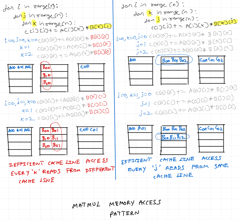
As seen above, memory access pattern for matrix B is inefficient on the left. Just by changing iteration order, access pattern for matrix B is fixed and we get free performance boost. Thus, having mechanical sympathy for the underlying hardware architecture helps in improving matmul performance.
LMAX Disruptor
When announced in early 2010s it made rounds in Java world and in HPC trading firms. It was also later adopted in Log4j and also in Nasdaq. Exchanges and brokerages workloads demand millisecond and microsecond latencies. They usually run on beefy bare-metal hardware as performance impact of running on VMs is too costly. These services are written in Thread per Core model (because context switching and L1, L2 cache invalidations are expensive) unlike traditional web-servers that operate on Thread per Request model.
Note: LMAX Disruptor is a high performance inter-thread communication library. Using it in a wrong way can cause significant performance degradation. Generally as a rule of thumb, if a problem can be solved just by scaling out instead of scaling up, it need not be used.
Here is a high level overview of LMAX Exchange.
The problem with traditional queues

The above diagram shows high level LMAX system receiving market data, doing auxiliary processing, core business logic processing and then sending orders to market. Replicator, Journaller & Un-Marshaller can process in parallel, but queues are still needed for ordered processing. So, we have receiver acting as producer and replicator, journaller & un-marshaller acting as consumers contending over shared resource - Queue.


As we saw in matmul section, it is more likely that tail & head vars fall within the same cache line. Producer thread is adding at the end of the queue and consumer thread is consuming from beginning of the queue. When threads are running in different cores, both their L1 & L2 caches needs to be invalidated each time producer / consumer is updating the state of the queue. LMAX team observed that their producer & consumer were running at the same rate & significant time was spent on keeping the L1 & L2 caches up-to date rather than doing actual producing & consuming.
How LMAX Disruptor is so Fast
Lock-Free RingBuffer
RingBuffer (CircularQueue) is also a Queue which operates in FIFO fashion. Key difference between RingBuffer & a traditional Queue is:
When values are consumed, it is not removed.
When end of the queue is reached, writer goes to the beginning of the queue and value is overwritten.
In LMAX Disruptor's RingBuffer implementation, the 'head' & 'tail' are managed outside the buffer instead of using a blanket lock which prevents adding value to end of the queue when consumption is happening in the beginning of the queue & vice versa.

Let's look at the highlighted sequence snapshot in the above diagram.
1) Fast consumer 2 has processed until buffer location 5 & asks cursor for next location. Cursor provides location 6, as location 0 is already processed by consumer 2. Consumer 2 fetches value in buffer location 6 and starts processing.
2) Producer barrier that is tracking consumer 1 & 2 sequences is aware that, consumer 1 is done only until buffer location 1, and consumer 2 is done until buffer location 5. So, only value at location 0 can be overwritten.
3) Producer can write only one value at location 0. Producer is preparing new value. Eg: Fetching latest value from network for example
4) Once new value is ready, producer asks producer barrier to commit. Value is updated in buffer, and sequence is updated to 7 from 0.
5) Slow consumer 1 that is done with processing buffer location 1, asks for next value. It gets the location 7 from cursor. Consumer 1 gets all entries in location 3-7 and works on processing it.
Consumers update their respective consumer sequences after processing. Only when a buffer location is processed by all consumers, it can be overwritten. Producer barrier keeps track of all consumer sequences.
Batching can be done in producer and consumer sequences (not in scope of this post, see references).
Buffer sequences are monotonically increasing as it provides an easier way of tracking consumer and producer buffer locations.
Static Memory Allocation & Delayed Garbage Collection
RingBuffer array is statically allocated with dummy values. Producers write to the next available buffer location using cursor and consumers consume previously unconsumed buffer locations using cursor. Once the value is overwritten there won't be any reference to it and will be easily garbage collected (GC).
In Java 8, GC there are 4 memory spaces. Young Generation (Eden, Survivor) spaces, Old Generation (Tenured Generation), Metaspace (non-heap memory) & Code Cache (JIT compiler related).
Since RingBuffer itself is statically allocated, it will be metaspace and will not be GC'd. The values in buffer are written and consumed quickly and will be GC'd in Eden cycle (quick and cheap), hence avoiding large GC pauses (survivor and old-gen spaces).
Avoiding False Sharing in Cache Lines
In matmul, we saw that variables in a program can share the same cache line. In Disruptor, we have Cursor, Sequence Barriers for both Producer & Consumers. Since we want producer and consumer threads to not be affected by updates to their variables (unlike ArrayBlockingQueue), we have to add padding so that the variable occupy entire cache line. So when producer is updating cursor, consumer caches need not be refreshed.

If we don't do this when producer thread updates cursor, consumer caches needs to be refreshed as they share the same cache line. This is called as False Sharing .
Java 8 has Contended Annotation for this.
Producer & Consumer Sequence Barriers
CPU core does several optimizations using instruction pipelining, reordering etc., as long as the outcome of a reorder or concurrent execution in execution units of a CPU core, doesn't change the outcome of the program.
Java provides Volatile keyword which is a special type of barrier know as write / store barrier. There are also other types of memory barriers and fences.
Here we have two programs where counter is not volatile and counter is volatile. We know that arithmetic operations happen in ALU of CPU core. Core operates using values from registers.
In first program, once counter is loaded into register, 10 iterations of loop happens and each change in counter value is saved only in register. Once the iteration is done, during "write-back" cycle, value is copied and written back to L1 cache and memory unit takes care of propagating this change to other levels of caches and to main memory.
public class LoopCounterExample {
    public static void main(String[] args) {
        int iterations = 10;
        int counter = 0;

        for (int i = 0; i < iterations; i++) {
            counter++;
        }
    }
}
public class LoopCounterExample {
    public static void main(String[] args) {
        int iterations = 10;
        volatile int counter = 0;

        for (int i = 0; i < iterations; i++) {
            counter++;
        }
    }
}
In second program, every update to counter is written back from Register to L1 cache and memory unit takes care of invalidating any other reference to this value. This has significant performance cost, but comes at the value of shared state across multiple threads.
In case of Disruptor, Cursor, Consumer sequences & Producer sequences use memory barrier & fences which offer finer control than volatile keyword. This is done using Java VarHandle.
These techniques offer finer control than Reentrant Lock used in ArrayBlockingQueue. Producer and Consumers can write and consume from ring-buffer at the same time ,and can be confident that when value is read from a buffer location it is always the latest because barriers & fences guarantee:
Anything that happened before barrier call is flushed out (producer adding newly produced value at location 0 and then incrementing cursor from 6 to 7).
Value updated by one thread is immediately visible to all threads (value of cursor to consumer barrier and value consumer sequences producer barrier).
Avoiding Context Switching
Even without the below optimizations Disruptor's performance is significantly higher than an ArrayBlockingQueue (see perf benchmark section below). I found these optimizations very interesting (feel free to skip this and jump to perf section). These were done for LMAX matching engine service that has:
1 Inbound Disruptor with 1 producer and three consumers threads
3 Outbound Disruptor with 1 producer thread (one of the consumer threads from Inbound Disruptor) and 3 consumer threads.
Yellow arrows indicate critical threads that needs dedicated CPU core (for peak performance)

$ isolcpus=0,2,4,6,8,24,26,28,30,32
To isolate CPUs. Above diagram shows 10 cpu cores (20 hyper-threads) isolated from OS kernel scheduler. OS will not schedule any process or thread in these cores. (Plugging my previous post here if you want to understand cpu cores and hyper-threading)
$ cset set --set=/system --cpu=18,20,...,46
$ cset set --set=/app --cpu=0,2,...,40
To partition system resources. Separate cpu sets for system and app
$ cset proc --move -k --threads --force \ --from-set=/ --to-set=/system
This command moves kernel threads from the default CPU set to the "/system" CPU set. Kernel threads are system-level threads managed by the kernel itself.
$ cset proc --exec /app \ taskset -cp 10,12...38,40 \ java <args>
This command executes the Java application (java ) within the CPU set "/app" using the taskset command. The taskset -cp option specifies which CPUs the process should be allowed to run on. In this case, the Java application is allowed to run on CPUs 10, 12, ..., 38, and 40.
sched_set_affinity(0);
sched_set_affinity(2);....
Each Java thread is pinned to dedicated core in application code.
Performance Benchmark
I've briefly covered principles and techniques through which LMAX disruptor gives performance gains. I would like to call out that I've used a mix of Disruptor 1.0 & 2.0 terminologies above to easily communicate the problem and underlying principles. For more detailed understanding, see sources in reference section.


Source: LMAX perf test Throughput & Latency. The above benchmarks were done without context switching optimizations.
Thus, having mechanical sympathy for the underlying hardware architecture helps to speed up inter-thread messaging and achieve peak performance.
Flash Attention
So far in this post, we looked at LOR using matmul & Disruptor and see how understanding underlying CPU architecture helps with extracting maximum performance. In this section, we'll look at Flash Attention - "A new attention algorithm that computes exact attention with far fewer memory accesses."
In my previous post, we understood HBM memory and compute intensity of A100 GPU using 2x2 matmul as an example. Flash Attention optimization leads to direct performance gains primarily in bandwidth & overhead bound rather than optimizations in compute bound regime.
As of April 2024, I don't have deep expertise / understanding to explain attention layer of Transformers in detail. Refer to Jay Alammar's amazing post or high quality video from 3Blue1Brown for that. I also cannot do a better job than Aleksa Gordi in explaining step-by-step changes in Flash Attention 1 algorithm with supporting math. Refer to his excellent post for that. Below, I try to provide a practical high level FlashAttention 1 explanation w.r.t underlying Hardware - CUDA Ampere Architecture.
Paper Title: Fast and Memory-Efficient Exact Attention with IO-Awareness
Exact Attention: It's not using sparse matrix / approximation methods to speed up attention calculation. These technique when used, result in models with poor quality. Flash Attention 1 uses exact attention calculation, so there is no reduction in quality.
Fast & Memory-Efficient: Space complexity of vanilla self-attention is O(N), while the algorithmic optimization leads to space complexity of N (O(N)). This reduction is space complexity results in increased memory bandwidth availability, decreasing compute intensity [more data is fed to the beast - CUDA & Tensor cores :) from caches], resulting in improvement in speed.
IO Awareness: NVIDIA A100 SXM GPU has 40-80 GB of HBM (VRAM / DRAM) & 88.1 MB of SRAM in total shared across all SMs (256k registers, 192k L1 cache per SM -> 27.8 MB for registers and 20.3MB for L1 cache combined + 40MB of shared L2 cache).

Diagram source is NVIDIA. It shows required Compute Intensity for FMA operation in CUDA & Tensor Cores - to make the read operations worth the cost. Except for matmul, there are not many computations that have such high compute intensity to make reads from slower memory worth the cost. So, model implementations must try to keep the compute intensity as low as possible. i.e, read and write from caches and registers.

Diagram source is Flash Attention paper. In above attention diagram, in native attention implementation in PyTorch, we can that only ~4ms out of 17ms is spent on Matmul operation (compute bound). The rest of the operations are not that compute heavy. But because of frequent read and writes from HBM, the bandwidth is significantly reduced resulting in wasted GPU compute cycles and higher latency.
Standard Self-Attention
I'm providing just a high level self-attention calculation operations needed to understand FlashAttention1. Refer 3Blue1Brown's video for detailed explanation.
Q1.K1 to Qn.Kn are matrix multiplication of Q&K matrices. The division is for numeric stability (not critical for this post).

The resulting values from matmul range from - infinity to + infinity.

Since matrix column values are used for predicting next token, we need a probability distribution. Softmax operation is applied to every column of the result embedding matrix. The denominator needs sum of all elements in a given column. See sample program below and results with help from ChatGPT.

import torch
import torch.nn.functional as F

def traditional_softmax(matrix, column_index):
    column = matrix[:, column_index]
    softmax_column = F.softmax(column, dim=0)
    return softmax_column

# Example usage
matrix = torch.tensor([[-0.8, -5.0, 5.0, 1.5, 3.4, -2.3, 2.5],
                       [-0.2,  2.3, 3.5, 1.8, 0.9, -1.5, 0.5]], dtype=torch.float32)
column_index = 2
softmax_result = traditional_softmax(matrix, column_index)
print("Softmax for column", column_index, ":", softmax_result)

# result
# Softmax for column 2 : tensor([0.8176, 0.1824])
The token with high probability score get's more "attention".

So far, we briefly saw matmul of matrices Q, K and softmax operation gives result matrix with probability distribution. Masking is applied before softmax to prevent next probability influencing previous token (refer video). Below we see outcome of result matrix after softmax is multiplied with V matrix.

This is how LLMs understand importance for words and sentences in different parts of the text. These steps are done for each layer of the model.
Below is the standard self-attention implementation which does above mentioned calculations for each input token in every layer of a transformer model.

Diagram source: Flash attention paper. One can quickly see, several reads and writes being done to HBM without taking bandwidth and compute intensity of underlying GPU architecture into account.
Flash Attention Optimizations

Diagram source: HuggingFace TGI
Tiled Matrix Multiplication
We are going to revisit.. caches ! (you guessed it :)) Refer to MIT OpenCourseWare matmul with tiling. This is the critical critical change


In the first slide, entire matrix B is loaded as all columns are needed. This is not very efficient use of memory bandwidth. As we saw earlier, In self-attention there are 3 matrix multiplications and one softmax (next section covers online softmax, so for now assume that not all columns are needed for softmax calculation).
Once tiling is done, some bandwidth in HBM is freed up, and some L1 & L2 cache memory are also freed up. This will be used to do softmax operation once Q.K for the block is done. Once softmax is done, we do another matrix multiplication with V block. This result is then written back to HBM. This is called as "Kernel Fusion". ie., a CUDA kernel is doing 3 operations.
A side note: I would imagine there was some kind of tiling already happening on transformer models before FlashAttention. Because, CUDA Thread Blocks & Warps are designed to do parallel operations on every memory page read. I haven't looked into FlashAttention 2, but from reading the abstract, I think this is being done. Again, this highly emphasizes the need for optimizations with Mechanical Sympathy :)
Online Softmax Calculation
Earlier we saw that softmax needs the sum of all elements in a given column. In online softmax calculation, computations are performed for columns in smaller matrix blocks, reducing the memory footprint in SRAM. With each block calculation in flash attention, the maximum score within the block is tracked and saved.
m(x) (Maximum Score): The highest value within a block of scores.
f(x) (Exponential Function): Transforms scores into positive values by raising them to the power of the difference between the score and the maximum score across all blocks resulting in numerical stability
l(x) (Sum of Exponential Scores): The sum of exponential values obtained from applying the exponential function to each score within a block, used for softmax probability computation.
See sample program and results with help from ChatGPT.
import torch
import torch.nn.functional as F

def flash_attention_softmax(matrix, column_index, block_sizes):
    # Step 1: Extract the column vector
    column = matrix[:, column_index]

    # Step 2: Compute the total size of the concatenated vector
    total_size = column.size(0)

    # Step 3: Split the concatenated vector into blocks
    blocks = torch.split(column, block_sizes)

    # Step 4: Compute the maximum value within each block (𝑚(𝑥))
    max_values = [torch.max(block) for block in blocks]

    # Step 5: Compute the global maximum value across all blocks
    global_max = torch.max(torch.stack(max_values))

    numerator = torch.zeros_like(column)
    for i, block in enumerate(blocks):
        # Step 6: Compute numerator for each block (𝑓(𝑥))
        numerator[i * block_sizes[i]:(i + 1) * block_sizes[i]] = torch.exp(block - global_max)

    # Step 7: Compute the sum of exponentials (ℓ(𝑥))
    denominator = torch.sum(numerator)

    # Step 8: Compute softmax probabilities for each block
    softmax_probabilities = numerator / denominator

    return softmax_probabilities

# Example usage
matrix = torch.tensor([[-0.8, -5.0, 5.0, 1.5, 3.4, -2.3, 2.5],
                       [-0.2,  2.3, 3.5, 1.8, 0.9, -1.5, 0.5]], dtype=torch.float32)
column_index = 2
block_sizes = [1, 1]  # Splitting the column into individual elements

print("Matrix:")
print(matrix)

print("\nColumn:")
column = matrix[:, column_index]
print(column)

print("\nBlocks after splitting:")
blocks = torch.split(column, block_sizes)
print(blocks)

print("\nMax values within each block:")
max_values = [torch.max(block) for block in blocks]
print(max_values)

print("\nGlobal maximum value across all blocks:")
global_max = torch.max(torch.stack(max_values))
print(global_max)

softmax_result = flash_attention_softmax(matrix, column_index, block_sizes)
print("\nSoftmax for column", column_index, ":", softmax_result)int("Softmax for column", column_index, ":", softmax_result)

# Matrix:
# tensor([[-0.8000, -5.0000,  5.0000,  1.5000,  3.4000, -2.3000,  2.5000],
#         [-0.2000,  2.3000,  3.5000,  1.8000,  0.9000, -1.5000,  0.5000]])

# Column:
# tensor([5.0000, 3.5000])

# Blocks after splitting:
# (tensor([5.]), tensor([3.5000]))

# Max values within each block:
# [tensor(5.), tensor(3.5000)]

# Global maximum value across all blocks:
# tensor(5.)

# Softmax for column 2 : tensor([0.8176, 0.1824])
To summarize:

(Although I haven't gone into Transformer attention mechanism, math & Flash Attention algorithm, math; I am hoping that at a high level, I was able to communicate the essence of Flash Attention 1 optimizations.)
Tri Dao, et al., with their combined research / expertise & very good understanding in:
Transformer Attention mechanism and the math behind it
NVIDIA Ampere series GPU architecture & CUDA parallel programming
Earlier research works - Self-attention Does Not Need O(n2) Memory by Google Researchers with reference implementation in JAX for TPU & Online normalizer calculation for softmax by NVIDIA researchers with reference implementation in CUDA
have shown Mechanical Sympathy to extract the best out of NVIDIA Ampere GPU hardware architecture.
Outro
Implementing matmul of 4096x4096 in C and changing loop order provides 461% improvement in GFLOPS utilization compared to C implementation with inefficient loop order. This is done purely by exploiting CPU cache line behavior.
P99 latency % improvement when comparing Disruptor against ArrayBlockingQueue is 99% & enabled LMAX Exchange to handle 6M order matching engine TPS on a single machine. This is done primarily by using granular inter-thread messaging allowing concurrent read and writes to buffer, and efficient use of CPU cache line.
FlashAttention trains Transformers faster than existing baselines: 15% end-to-end wall-clock speedup on BERT-large (seq. length 512) compared to the MLPerf 1.1 training speed record, 3 speedup on GPT-2 (seq. length 1K), and 2.4 speedup on long-range arena (seq. length 1K-4K)
In this post, we saw examples of Mechanical Sympathy being applied in wide range of problems requiring different skill-sets and expertise with real world impact.
Deep Learning space is still in its nascent phase. People with expertise in several background (Data Engineering, Model Training, Deep Learning Algorithms, Compiler, Hardware Interface - CPUs, GPUs, Accelerators, Model Inference, Distributed Systems, Infrastructure, Mathematics, Physics, Chemistry) are all working within their domain and rightfully so. Current cost of training & inference for quality models is prohibitively high. Given how LLMs are going to be human companions like a Laptop and a smartphone, several optimizations will be required and some of which will be solved by engineers having very good understanding of underlying hardware and architecture.
It's interesting that FlashAttention 1 was done in 2-3 months. In 2023, they've also published Flash Attention 2 with better parallelism and work partitioning (efficient use of CUDA thread blocks & warps) resulting in optimizations primarily in compute bound regime. I cannot imagine the breakthroughs we would see - If more DeepLearning / Transformer algorithm experts/researchers and CUDA Architects like Stephen Jones, work on optimizing existing layers and algorithms for couple years or so. I'm highlighting CUDA here as NVIDIA is the market leader. Intel, AMD, and other transformer accelerators' computing platform teams should also be spending more effort on optimizing model implementations for their respective hardware.
References:
MIT OpenCourseWare - Performance Engineering - Matrix Multiplication https://youtu.be/o7h_sYMk_oc?si=mWgShE48VgXARZEz
Vipul Vaibhaw's MIT matmul summary - https://vaibhaw-vipul.medium.com/matrix-multiplication-optimizing-the-code-from-6-hours-to-1-sec-70889d33dcfa
Tao Xu's MIT matmul summary - https://xta0.me/2021/07/12/MIT-6172-1.html
InfoQ Martin Thompson and Michael Barker on building HPC fintech handling over 100k TPS at LMAX - https://www.infoq.com/presentations/LMAX
InfoQ Sam Adams on LMAX Exchange Architecture https://www.infoq.com/presentations/lmax-trading-architecture/
Trisha Gee on LMAX Disruptor Internals - RingBuffer, LocksAreBad, MemoryBarriers, Consumer, Producer, Disruptor 2.0
LMAX Exchange Disruptor - https://lmax-exchange.github.io/disruptor/#_read_this_first
Martin Thompson on Memory Barriers & Fences - https://mechanical-sympathy.blogspot.com/2011/07/memory-barriersfences.html
Guy Nir on LMAX Disruptor - https://www.slideshare.net/slideshow/the-edge-2012-disruptor-guy-raz-nir-published/22790571
Martin Fowler on LMAX Disruptor: https://martinfowler.com/articles/lmax.html
Tri Dao, et al., FLASH ATTENTION 1 & 2: https://github.com/Dao-AILab/flash-attention
Aleksa Gordi on ELI5 - FLASH ATTENTION 1: https://gordicaleksa.medium.com/eli5-flash-attention-5c44017022ad
Jay Alammar - The Illustrated Transformer


Top comments (0)