In the dynamic world of financial markets, staying ahead of the curve is crucial for investors. One key aspect of this is the ability to forecast stock prices accurately. In this blog post, we dive into the world of stock price forecasting by examining the performance of 59 Turkish stocks listed in İş Yatırım's Stock Tracking and Recommendation List. We will explore how well Auto ARIMA, an automated time series forecasting technique, stands up to the challenge of predicting stock price movements in the Turkish market.
We will conduct a time series forecasting study using data spanning from January 2013 to August 2023. The objective of this study is to generate monthly forecasts for each month within this timeframe. The initial forecast will commence from the 24th month in the dataset, and subsequently, a new forecast will be generated for each consecutive month.
Import necessary libraries:
import yfinance as yf
import pandas as pd
import numpy as np
import time
from pmdarima import auto_arima
from sklearn.metrics import mean_squared_error
import matplotlib.pyplot as plt
plt.style.use('fivethirtyeight')
In this step, we import the required Python libraries for data collection, manipulation, time management, Auto ARIMA modeling, and performance evaluation.
Define stock tickers and date range:
tickers = [
    'AEFES',
    'AKCNS',
    'ARCLK',
    'ASELS',
    'BIMAS',
    'BIZIM',
    'CCOLA',
    'DOAS',
    'ENJSA',
    'ENKAI',
    'EREGL',
    'FROTO',
    'GWIND',
    'IPEKE',
    'KOZAA',
    'KOZAL',
    'KRDMD',
    'LOGO',
    'MAVI',
    'MGROS',
    'MPARK',
    'OTKAR',
    'OYAKC',
    'PETKM',
    'PGSUS',
    'SELEC',
    'SOKM',
    'TAVHL',
    'TCELL',
    'THYAO',
    'TKFEN',
    'TOASO',
    'TTKOM',
    'TTRAK',
    'TUPRS',
    'ULKER',
    'VESBE',
    'VESTL',
    'YATAS',
    'AKGRT',
    'ANHYT',
    'ANSGR',
    'TURSG',
    'AKBNK',
    'ALBRK',
    'GARAN',
    'HALKB',
    'ISCTR',
    'TSKB',
    'VAKBN',
    'YKBNK',
    'EKGYO',
    'ISGYO',
    'OZKGY',
    'TRGYO',
    'AGHOL',
    'ALARK',
    'KCHOL',
    'SAHOL'
]

start_date = '2013-01-01'
end_date = '2023-08-31'
Here, we define a list of 59 stock tickers representing Turkish companies. We also specify the start and end dates for collecting historical stock price data.
Create an empty DataFrame for predictions:
pred_df = pd.DataFrame(columns=['Date', 'Ticker', 'Adj Close', 'Prediction'])
We initialize an empty DataFrame called pred_df with columns for the date, stock ticker, actual adjusted closing price (Adj Close), and the predicted price (Prediction). This DataFrame will store our forecasting results.
Loop through each ticker and perform Auto ARIMA forecasting:
for ticker in tickers:
    data = yf.download(
        f'{ticker}.IS',
        start=start_date,
        end=end_date,
        interval="1mo",
        progress=False
    )
In this loop, we iterate through each stock ticker and use the Yahoo Finance API (yf.download) to download historical monthly stock price data for the specified date range. The data is stored in the data DataFrame.
Data preprocessing:
for ticker in tickers:
    data = yf.download(
        f'{ticker}.IS',
        start=start_date,
        end=end_date,
        interval="1mo",
        progress=False
    )

    data = data.reset_index()
    data = data[['Date', 'Adj Close']]

    data = data.dropna()

    first_data_date = data.iloc[0]['Date']
Here, we reset the index of the data, retain only the 'Date' and 'Adj Close' columns, remove any rows with missing data, and store the date of the first available data point in first_data_date.
Generate predictions:
for ticker in tickers:
    data = yf.download(
        f'{ticker}.IS',
        start=start_date,
        end=end_date,
        interval="1mo",
        progress=False
    )

    data = data.reset_index()
    data = data[['Date', 'Adj Close']]

    data = data.dropna()

    first_data_date = data.iloc[0]['Date']

    for i in range(24, len(data)):
        train_data = data[:i]
        test_data = data[i:i+1]

        model = auto_arima(train_data['Adj Close'], max_order=None, stepwise=True)
        prediction = float(model.predict(n_periods=1, return_conf_int=False))

        temp_df = pd.DataFrame({
            'Date': [test_data['Date'].values[0]],
            'Ticker': [ticker],
            'Adj Close': [test_data['Adj Close'].values[0]],
            'Prediction': [prediction]
        })
        pred_df = pd.concat([pred_df, temp_df], ignore_index=True)

        print(f'{ticker}: {i}')
This is the heart of the code. For each stock, we loop through the available data starting from the 24th month. We create a training dataset (train_data) containing historical price data and a test dataset (test_data) containing the price to be predicted. We then use the auto_arima function to fit an Auto ARIMA model to the training data and generate a one-month-ahead forecast (prediction). The results are appended to the pred_df DataFrame.
Sleep between requests:
for ticker in tickers:
    data = yf.download(
        f'{ticker}.IS',
        start=start_date,
        end=end_date,
        interval="1mo",
        progress=False
    )

    data = data.reset_index()
    data = data[['Date', 'Adj Close']]

    data = data.dropna()

    first_data_date = data.iloc[0]['Date']

    for i in range(24, len(data)):
        train_data = data[:i]
        test_data = data[i:i+1]

        model = auto_arima(train_data['Adj Close'], max_order=None, stepwise=True)
        prediction = float(model.predict(n_periods=1, return_conf_int=False))

        temp_df = pd.DataFrame({
            'Date': [test_data['Date'].values[0]],
            'Ticker': [ticker],
            'Adj Close': [test_data['Adj Close'].values[0]],
            'Prediction': [prediction]
        })
        pred_df = pd.concat([pred_df, temp_df], ignore_index=True)

        print(f'{ticker}: {i}')

    pred_df.loc[pred_df['Ticker'] == ticker, 'First Data Date'] = first_data_date

    time.sleep(1)
Finally, we update the 'First Data Date' column in pred_df with the first available data date for each stock and add a one-second pause between requests to avoid overloading the Yahoo Finance servers during data collection.
This code allows for systematic and data-driven stock price forecasting for the selected Turkish stocks, producing predictions for each month within the specified date range.

In the realm of stock price forecasting, evaluating the accuracy of predictions is essential for investors and analysts alike. One commonly used metric for assessing the quality of predictions is Root Mean Squared Error (RMSE). RMSE provides valuable insights into the degree of error between predicted values and actual outcomes, offering a quantitative measure of the forecasting model's performance.
RMSE quantifies the average magnitude of errors by taking the square root of the mean of the squared differences between predicted values and observed (actual) values. A lower RMSE signifies a closer alignment between predictions and reality, indicating a more accurate forecasting model.
In the following analysis, we employ RMSE as a key performance metric to assess the accuracy of our stock price predictions for a diverse portfolio of Turkish stocks. Each stock's RMSE will shed light on the reliability of our forecasting model, helping us identify strengths and areas for improvement in our predictive capabilities.
Creating an empty RMSE (Root Mean Squared Error) dictionary:
rmse_dict = {}
In this step, we initialize an empty dictionary to store the root mean squared error (RMSE) for each stock symbol's predictions. The dictionary will store RMSE values for each stock symbol.
Calculating RMSE for each stock symbol:
for ticker in tickers:
    ticker_data = pred_df[pred_df['Ticker'] == ticker]

    actual_values = ticker_data['Adj Close'].values
    predicted_values = ticker_data['Prediction'].values

    rmse = np.sqrt(mean_squared_error(actual_values, predicted_values))
    rmse_dict[ticker] = rmse
This loop calculates the RMSE value for each stock symbol. First, we select the relevant predictions for the specific stock symbol from the pred_df DataFrame and store them in the ticker_data DataFrame. Then, we extract the actual values (actual_values) and predicted values (predicted_values) from this subset.
RMSE is calculated as the square root of the mean of the squared errors between the actual and predicted values. The mean_squared_error function calculates these errors, and we find the RMSE by taking the square root using np.sqrt.
Finally, we add the calculated RMSE value for each stock symbol to the rmse_dict dictionary. This allows us to evaluate how accurate or inaccurate the predictions are for each stock symbol. RMSE is a crucial metric for measuring how close the predictions are to the actual values.
Sorting RMSE values in ascending order:
sorted_rmse_dict = dict(sorted(rmse_dict.items(), key=lambda item: item[1]))
In this step, we create a new dictionary called sorted_rmse_dict. We sort the rmse_dict dictionary based on the RMSE values in ascending order. This sorting is achieved using the sorted function, which takes each item in the dictionary and sorts them based on the RMSE values (item[1] represents the value in each dictionary item). The result is a dictionary containing the stock tickers as keys and their RMSE values in ascending order.
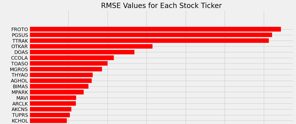
Creating a horizontal bar chart:
plt.figure(figsize=(12, 16))
plt.barh(list(sorted_rmse_dict.keys()), list(sorted_rmse_dict.values()), color='red')
plt.xlabel('RMSE Value')
plt.ylabel('Stock Ticker')
plt.title('RMSE Values for Each Stock Ticker')
plt.tight_layout()
plt.show()

In this step, we create a horizontal bar chart to visualize the RMSE values in ascending order. The plt.figure function defines the figure size, and plt.barh creates the horizontal bar chart. We use the keys (stock tickers) from the sorted_rmse_dict as the y-axis labels and the corresponding RMSE values as the bar lengths. The bars are colored in red for better visibility. We add labels for the x-axis and y-axis, and a title for the chart. Finally, plt.show() displays the chart.
This visualization allows us to compare the RMSE values for each stock ticker in ascending order, helping us identify which stocks have the most accurate predictions and which ones have higher prediction errors.
In conclusion, this blog post shows how automated time series forecasting techniques can be used in financial markets and underlines the significance of assessing prediction accuracy. It also emphasizes the importance that solutions like Auto ARIMA may provide to investors and analysts. However, it's important to remember that prediction accuracy varies each stock, underscoring the importance of diligent portfolio management.
What really counts? The forecasts or a thorough examination of the forecasts?
Voices That Matter: Discover User Comments Below

Please correct me if I misunderstand. The last bar chart seems to calculate RMSE values in absolute values; if you normalize it, the comparison will be more accurate, for example, this value for FROTO is actually due to the share price being too high.

When you perform the analysis for BIST (Borsa İstanbul) stocks using MAPE with Auto-ARIMA, what is the situation like?
"MAPE is a measure of how accurate the forecast is. MAPE calculates the percentage difference between the actual value and the forecast. The smaller the MAPE, the more successful the forecast."


Top comments (0)