Learning how to perform Twitter Sentiment Analysis

Keras challenges the Avengers

Sentiment Analysis, also called Opinion Mining, is a useful tool within natural language processing that allow us to identify, quantify, and study subjective information. Due to the fact that quintillion of bytes of data is produced every day, this technique gives us the possibility to extract attributes of this data such as negative or positive opinion about a subject, also information about which subject is being talked about and what characteristics hold the persons or entities expressing that opinion.

Twitter has been growing in popularity and nowadays, it is used every day by people to express opinions about different topics, such as products, movies, music, politicians, events, social events, among others. A lot of movies are released every year, but if you are a Marvel’s fan like I am, you’d probably be impatient to finally watch the new Avengers movie. Personally, I want to know how the people is feeling about this.

Previously, we have discussed how we can use the Twitter API to stream tweets and store them in a relational database. Now, we will use that information to perform sentiment analysis. But before that, we should take into consideration some things. First of all, we have streamed our tweets using the term ‘Avengers’ but without any extra consideration. It is highly likely that we have thousands of repeated tweets. In terms of sentiment analysis, processing them will not add any extra value and contrary, it will be computationally expensive. So, we need to access the database and delete duplicated tweets keeping the first occurrence. Second, we have an unlabeled database. For the model to learn during training, we should state if the tweets are positive or negative. The ideal solution would be to manually label the dataset, which is very accurate but requires a lot of time. However, there are several alternatives such as using an open-source dataset labeling tool such as Stanford CoreNLP.

There are a high number of frameworks that can be used for machine learning tasks, however, we are going to use Keras because it offers consistent and simple APIs, minimizes the number of user actions required and more importantly, it is easy to learn and use. We will also make use of the Natural Language Toolkit (NLTK), that provides many corpora and lexical resources that will come in handy for tagging, parsing, and semantic reasoning, and Scikit-learn, that provides useful tools for data mining and data analysis.

Ready to start? Let’s see what Keras can learn about Avengers.

First of all, we need to retrieve the tweets that we have previously store in our PostgreSQL database. For that aim, we are going to take advantage of sqlalchemy, a Python SQL toolkit and Object Relational Mapper that will allow us to connect and query the database in an easy way. One of the characteristics of sqlalchemy is that includes dialect (the system that it uses to communicate with databases) implementations for the most common database, such as MySQL, SQLite, and PostgreSQL, among others. We’ll use the create_engine() function that produces an Engine object based on a given database URL which typical form is as follows: dialect+driver://username:password @host :port/database. In our case, the dialect is PostgreSQL while the driver is psycopg2. After creating the engine object, we’ll use the function read_sql_query from pandas module to query the database to obtain all the data stored in our tweet table (‘select * from tweet_table’) and gather the information retrieved in a DataFrame:

Before we dig into analyzing the public opinion on ‘Avengers’, there is an important step that we need to take: preprocessing the tweet text. But what does this mean? Text preprocessing includes a basic text cleaning following a set of simple rules commonly used but also, advanced techniques that take into account syntactic and lexical information. In the case of our project, we are going to perform the following steps:

• Convert tweets to lowercase using **.lower() function**, in order to bring all tweets to a consistent form. By performing this, we can assure that further transformations and classification tasks will not suffer from non-consistency or case sensitive issues in our data.
• Remove ‘RT’ , UserMentions and links: In the tweet text, we can usually see that every sentence contains a reference that is is a retweet (‘RT’), a User mention or a URL. Because it is repeated through a lot of tweets and it doesn’t give us any useful information about sentiment, we can remove them.
• Remove numbers: Likewise, numbers do not contain any sentiment, so it is also common practice to remove them from the tweet text.
• Remove punctuation marks and special characters: Because this will generate tokens with a high frequency that will cloud our analysis, it is important to remove them.
• Replace elongated words: an elongated word is defined as a word that contains a repeating character more than two times, for example, ‘Awesoooome’. Replacing those words is very important since the classifier will treat them as different words from the source words lowering their frequency. Though, there are some English words that contain repeated characters, mostly consonants, so we will use the wordnet from NLTK to compare to the English lexicon.
• Removing stopwords : Stopwords are function words that are high frequently present across all tweets. There is no need for analyzing them because they do not provide useful information. We can obtain a list of these words from NLTK stopwords function.
• Handling negation with antonyms : One of the problems that come out when analyzing sentiment is handling negation and its effect on subsequent words. Let’s take an example: Say that we find the tweet “I didn’t like the movie” and we discard the stopwords, we will get rid of “I” and “didn’t” words. So finally, we will get the tokens “like” and “movie”, which is the opposite sense that the original tweet had. There are several ways of handling negation, and also there is a lot of research going on about this; however, for this project, in particular, we are going to scan our tweets and replace with an antonym (that we’ll get from lemmas in wordnet) of the noun, verb or adjective following our negation word.

After we have cleaned our data but before we start building our model for sentiment analysis, we can perform an exploratory data analysis to see what are the most frequent words that appear in our ‘Avengers’ tweets. For this part, we will show graphs regarding tweets labeled as positive separated from those labeled as negative.

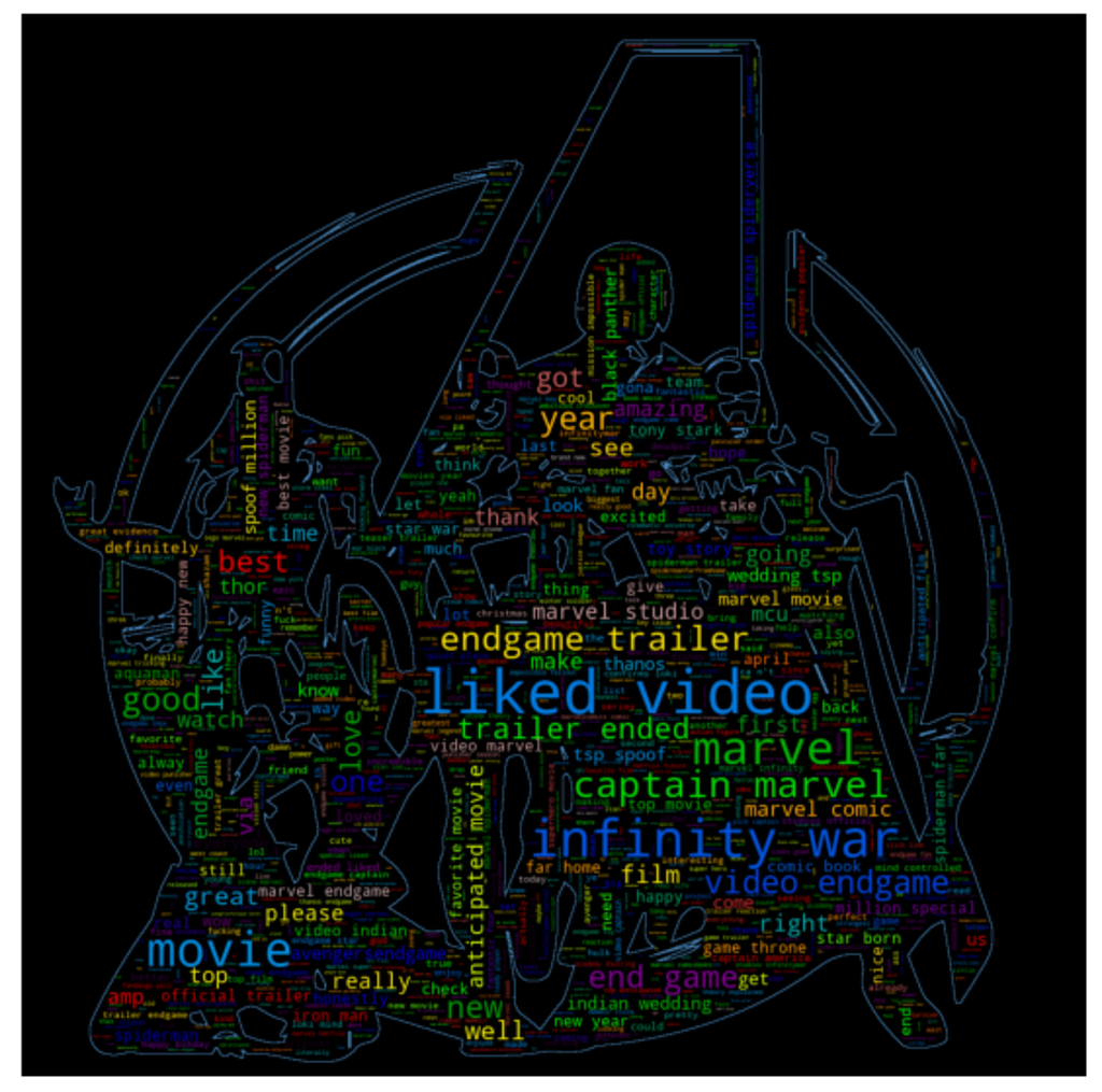
We will start by using WordCloud to represent the word usage across all tweets by resizing every word proportionally to its frequency. Even though it would seem not the most appropriated for different reasons, this graph provides a textual analysis and a general idea of which type of words are present more frequently in our tweets. Python has a WordCloud library that allows us to apply a mask using an image that we upload from our hard drive, select the background, the word colormap, the maximum words, font size, among other characteristics of the graph.

WordCloud for positive tweets:

WordCloud for negative tweets:

When we observed the WordCloud for positive tweets, some of the words that appear in a bigger size do not have a particular connotation and can be interpreted as neutral, such as “Captain Marvel”, “infinity war”. On the other hand, other words, even though some of smaller size, could be explained to be in tweets with a positive sense, such as “good”, ”great”, ”best” and “liked”. On the contrary, WordCloud for negative tweets showed mostly neutral words such as “movie”, “endgame” and very small words with a negative connotation, for example, “never”, and “fuck”.

Afterward, we can present in a graph the 50 most frequent words in co-occurrence with ‘Avengers’ term for positive and negative tweets. We’ll start by using the function CountVectorizer from sklearn which will convert the collection of tweets into a matrix of token counts producing a sparse representation of the counts. Then, we sum all counts for each token and obtain the frequency and store them as a DataFrame.

We can now plot these values in a barplot by using matplotlib function bar.

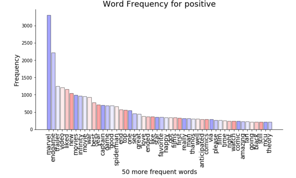
We can see that the first frequent words are common for positive and negative tweets: “marvel”, “endgame” and moreover, most of the words have a neutral connotation, except for words like “good”, “great”, “love”, “favorite” and “best” in the positive tweets.

We can finally check if there is any correlation between the frequency of the words that appear in the positive and negative tweets. We’ll concatenate both word frequency DataFrames and after that, we’ll use the seaborn regplot graph:

Apart from one or two points that seem related, no meaningful association can be derived from the graph above between words appearing in positive and negative tweets.

After visualizing our data, the next step is to split our dataset into training and test sets. For doing so, we’ll take advantage of the train_test_split functionality of sklearn package. We will take 20% of the dataset for testing following the 20–80% rule. From the remaining 80% used for the training set, we’ll save a part for validation of our model.

We also need to convert our sentiment column into categories that our model can understand. We’ll use then 0 for negative, 1 for neutral and 2 for positive tweets.

Finally, we need to process our input tweet column using TfidfVectorizer that will convert the collection of tweets to a matrix of Term Frequency/Invert document frequency (TF-IDF) features. What is very crucial about this function is that it will return normalized frequencies; feature normalization is a key step in building a machine learning algorithm. After several tries, 3500 was the number of maximum features returned that worked best with our model.

Now, it’s time to build our model: a neural network. If you are not familiar with how neural networks work, you can check my previous post. Fortunately, Keras makes building a neural network very simple and easy in a few lines of code.

Let’s dissect our model: Sequential() is a type of network composed of layers that are stacked and executed in the order presented. So, which type of layers do we have? We observe that we have added Dense layers for our three layers (input, hidden and output layer), meaning that every node in a layer receives input from all nodes in the previous layer implementing the following operation: output = activation(dot(input, weights) + bias). Between them, we have used the Dropout method, which takes a float between 0 and 1 (that we’ll pass as drop and adjust later) representing the fraction of the neurons that will be randomly dropped during training to prevent overfitting. The key layers are the input and the output because they will determine the shape of our network and it is important to correctly know what we expect. Because we’ll use 3500 as the maximum features returned in the vectorization process, we need to use this exact number as the size of the input shape. We’ll also include how many outputs will come out of the first layer (pass as layer1), a parameter that we‘ll modify later in order to make the layer simpler or more complex. In this case, we’ll choose relu as our activation function, which has several benefits over others such as reducing the likelihood of vanishing gradient. For the last layer, we’ll choose three nodes corresponding to the three different outputs and because we want to obtain categorical distributions, we’ll use softmax as an activation function. For the hidden layer, we’ll also pass the size as layer2 that normally is half layer1 and because it's a classification problem, we'll use sigmoid activation (if you want to know more about which activation functions to use, check this video).

After that, the optimizer to be used and its parameters should be stated. We’ll use AdamOptimizer with fixed decay and betas, but later we’ll adjust the learning rate and epsilon value. Adam is a stochastic optimization which has several advantages such as being straightforward to implement, being computationally efficient, having little memory requirements, being invariant to diagonal rescaling of the gradients, and being well suited for problems that are large in terms of data and/or parameters.

One of the last steps before training is to compile the network clarifying the loss we want. In this case, we’ll use sparse_categorical_crossentropy due to the fact that we have categories represented as numbers. We’ll also need to clarify the optimizer, and the metrics to be evaluated (for us, it’ll be accuracy). Moreover, we need to fit the model stating the set for X and Y values, the batch size (number of samples propagated through the network), epochs (how many times we’ll scan through all the data, parameter that we’ll also adjust), the validation split (which percentage will be saved to validate our results) and if we are going to present the data every time in the same way or, we are going to shuffle it (shuffle).

After trying several parameters for dropout, features, shuffle, learning rate, layer size, epsilon, validation_split, epochs, we’d finally arrived at the following model:

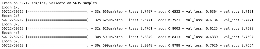
We can see that our final validation accuracy was 71.91 seen for epoch 1 improving to 76.54% for epoch 5. Furthermore, increasing, even more, the epochs improved the training accuracy but decreased the validation accuracy.

Even though we always want to have higher accuracy, we can now go on and try to identify what the opinion is in a new dataset that we have created just like the one we used for training and validation.

For that, we are going to query our new database, performed the same text preprocessing step, tokenize our tweets and use our trained model to predict the sentiment on ‘Avengers’ using model.predict(). If we want to make it easier for human readability, we can convert the numeric prediction to our categorical labels ‘positive, neutral and, negative’.

Now the time of the truth! We can plot how many of our tweets are including in each sentiment category using a pie chart:

As you can see 53.1% of the tweets have a positive connotation about ‘Avengers’ while the remaining 46.9% are neutral or have a negative connotation. If I was to tweet about this subject I should be included on the positive side, or a least I can be 76% confident I would. What about you?

Next, we are going to use Tweets information to visualize user interactions on Twitter by using NetworkX.

If you want to get to know the entire code for this project, check out my GitHub Repository.

---