Introduction

MindsDB is an open-source machine-learning tool that brings automated machine learning to your database. MindsDB offers predictive capabilities in your database. Tableau lets you visualize your data easily and intuitively. In this tutorial, we will be using MindsDB to predict the hourly electricity demand in the United States and visualize results in Tableau. To complete this tutorial, you are required to have a working MindsDB connection, either locally or via cloud.mindsdb.com. You can use this guide to connect to the MindsDB cloud.

Data Setup

Connecting the data as a file

Follow the steps below to upload a file to MindsDB Cloud.

• Log in to your MindsDB Cloud account to open the MindsDB Editor.
• Navigate to Add data the section by clicking the Add data button located in the top right corner.

• Choose the Files tab.
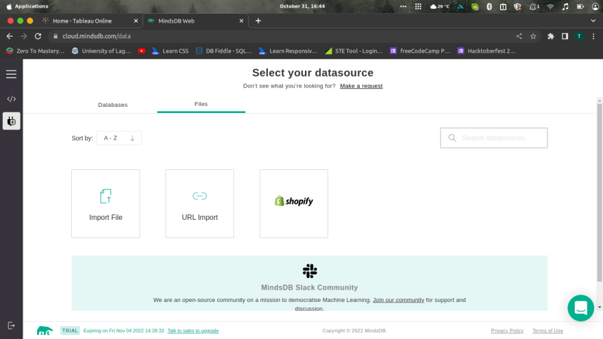
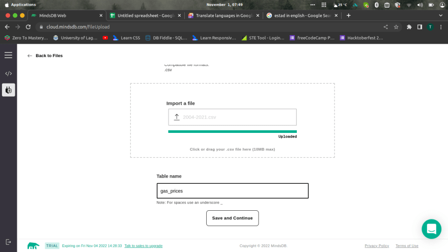
• Choose the Import File option.
• Upload a file (2004-2021.tsv), name a table used to store the file data (here it is gas_prices ), and click the Save and Continue button.

Once you are done uploading, you can query the data directly with the;

SELECT * FROM files.gas_prices LIMIT 10;

The output would be:

Understanding the Dataset

The National Agency of Petroleum, Natural Gas, and Biofuels (ANP in Portuguese) releases weekly reports of gas, diesel, and other fuel prices used in transportation across the country. These datasets bring the mean value per liter, the number of gas stations analyzed and other information grouped by regions and states across the country.

Note: The original dataset was written in Spanish and translated by me into English.

Context

• INITIAL DATE
• FINAL DATE
• REGION
• STATE
• PRODUCT
• Visted_Gas_Station
• Measure_Unit
• Resell_mean_price
• Standard_deviation
• Min_Resell_Price
• Max_Resell_Price
• Mean_Resell_Margin
• Resell_Variant_COEF
• Mean_Price_Distribution
• Standard_Deviation_Distribution
• Min_Price_Distribution
• Max_Price_Distribution
• Max_Price_Distribution

What can be done with this dataset?

• How different regions of Brazil saw their gas prices change?
• Within a region, which states increased more their prices?
• Which states are the cheapest (or most expensive) for different types of fuels?

In this tutorial, we will be predicting the mean_price_distribution.

Creating the Predictor

Let’s create and train the machine learning model. For that, we will use the CREATE PREDICTOR statement and specify the input columns used to train FROM(features) and what we want to PREDICT(labels).

Note: This is a timestamp series model

CREATE PREDICTOR mindsdb.[predictor_name]
FROM [integration_name]
    (SELECT [sequential_column], [partition_column], [other_column], [target_column]
     FROM [table_name])
PREDICT [target_column]

ORDER BY [sequential_column]
GROUP BY [partition_column]

WINDOW [int]
HORIZON [int];

• CREATE PREDICTOR: Creates a predictor with the name predictor_name in the mindsdb table.
• FROM files: Points to the table containing the data.
• PREDICT Close: Dictates the column to predict.
• ORDER BY: Shows the column to arrange the data during training.
• GROUP BY: It is optional. The column by which rows that make a partition are grouped. For example, if you want to forecast the inventory for all items in the store, you can partition the data by product_id, so each distinct product_idhas its own time series.
• WINDOW: Decides how many rows to "look back" into when creating a prediction.
• HORIZON: Specifies the number of future predictions. The default is 1.

Let’s proceed to make predictions on our dataset:

CREATE PREDICTOR mindsdb.gas_prices_brazil
FROM files
  (SELECT * FROM gas_prices)
PREDICT Mean_Price_Distribution
ORDER BY FINAL_DATE
GROUP BY REGION, STATE
-- the target column to be predicted stores one row per quarter
WINDOW 300     
HORIZON 100;    -- making forecasts for the next year (next 100 rows)

Status of a Predictor

A predictor may take a couple of minutes for the training to complete. You can monitor the status of the predictor by using this SQL command:

SELECT status
FROM mindsdb.predictors
WHERE name='hourly_electricity_demand';

If we run it right immediately after creating a predictor, we get this output:

+------------+
| status     |
+------------+
| generating |
+------------+

After a while you will get:

+------------+
| status     |
+------------+
| training   |
+------------+

And finally, this should be your output:

+------------+
| status     |
+------------+
| complete   |
+------------+

Making Predictions

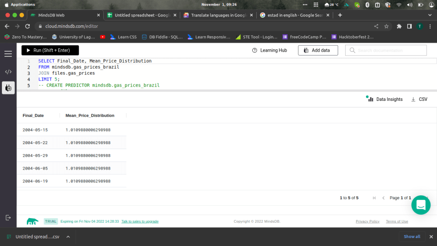
Now that we have our Prediction Model, we can simply execute some simple SQL query statements to predict the target value based on the feature parameters:

SELECT Final_Date, Mean_Price_Distrubution
FROM mindsdb.gas_prices_brazil
JOIN files.gas_prices
LIMIT 5;

Expected output would be:

Connecting MindsDB to Tableau

Tableau lets you visualize your data easily and intuitively. This tutorial will use Tableau to create visualizations of our predictions.

How to Connect

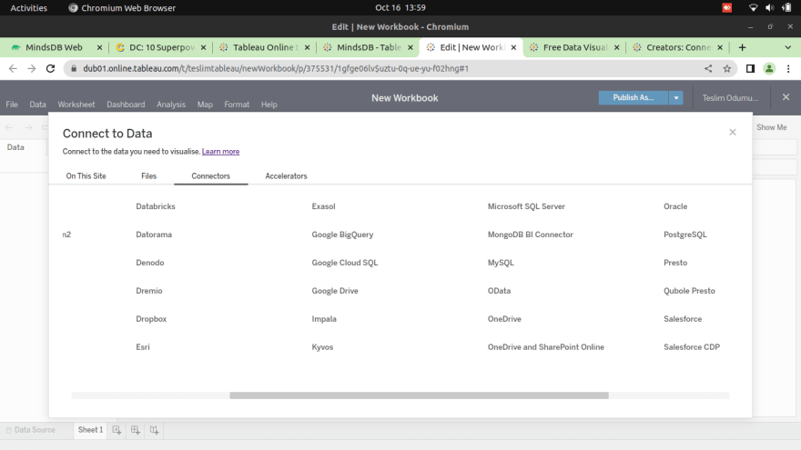
• First, create a new workbook in Tableau and open the Connectors tab in the Connect to Data window.
• Click on MySQL

• Input "cloud.mindsdb.com" for Server, "3306" for Port, "mindsdb" for Database "your mindsdb cloud email" for Username, "your mindsdb cloud password" for Password, and Sign in. Now you are connected and your page should look like this:

Visualizing our Data

Before you can visualize predictions in Tableau, you must first choose a data source. And because the predictions in this article are generated using a SQL statement, you will need to create a custom SQL query in Tableau to generate the data source. To do this:

• First, select the New Custom SQLon the left side of the window and use the query below to generate the mean price distributions for each date. You can preview the results or directly load the data into Tableau.

SELECT Final_Date, Mean_Price_Distrubution
FROM mindsdb.gas_prices_brazil
JOIN files.gas_prices

• Create an extract of the data under the connection heading at the top right of the window. You do this to facilitate data conversion to the appropriate data type. The extraction should take some time.

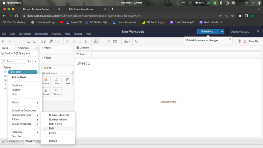
• Move to the Sheet tab on the bottom left and right-click the Mean_Price_Distribution and Date to convert their data types to Number(Decimal) and Date, respectively. Additionally, when right-clicking on the Mean_Price_Distribution and Final_Date, choose the option to convert it to a continuous measure.

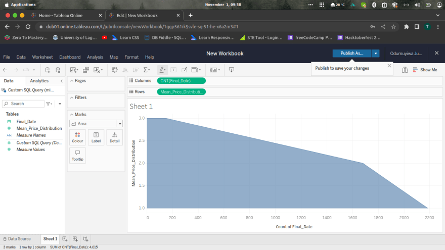
• Drag the Mean_Price_Distribution measure to the row shelf and the Final_Date dimension to the column shelf.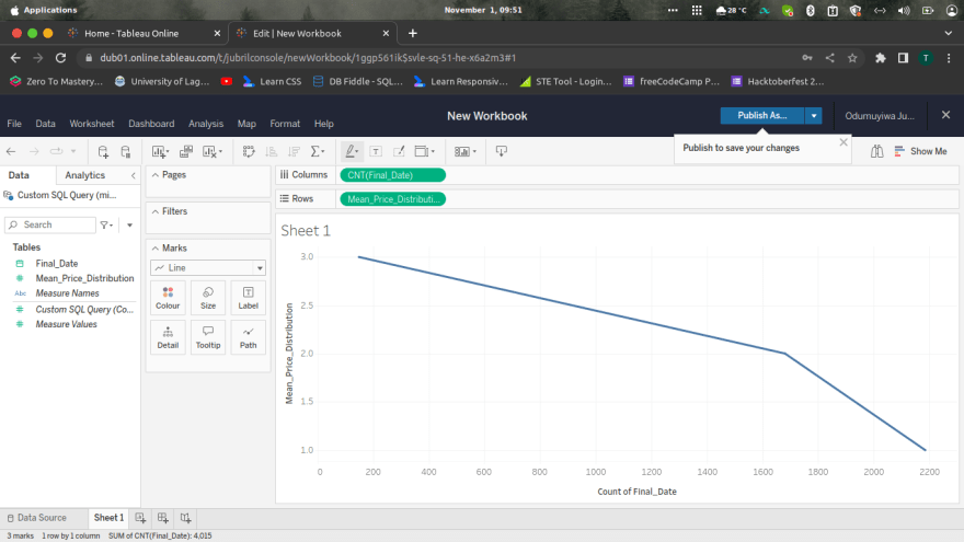
• You can also switch the visualization also to the line, area and etc.