Phase 2: Updating Your Prediction

From State to Sensors

While we were busy predicting, the GPS on our RC car was giving us positional data updates. These sensor measurements $\text{Z}_{t}$ give us valuable information about our world.

However, $\text{z}{t}$ and our state vector $\text{x}{t+1}$ may not actually correspond; our measurements might be in one space, and our state in another! For instance, what if we’re measuring our state in meters, but all of our measurements are in feet? We need some way to remedy this.

Let’s handle this by converting our state vector into our measurement space using an observation matrix H:

These equations represent the mean $μ{ₑₓₚ}$ and covariance $Σ{ₑₓₚ}$ of our predicted measurements.

For our RC car, we’re going from meters to feet, in both position and velocity. 1 meter is around 3.28 ft, so we would shape H to reflect this:

…leaving us with predicted measurements that we can now compare to our sensor measurements $\text{Z}_{t}$ . Note that H is entirely dependent on what’s in your state and what’s being measured, so it can change from problem to problem.

Our RC car example is a little simplistic, but this ability to translate our predicted state into predicted measurements is a big part of what makes Kalman filters so powerful. We can effectively compare our state with any and all sensor measurements, from any sensor. That’s powerful stuff!

An aside: The behavior of H is important. Vanilla Kalman filters use a linear Fₜ and H; that is, there is only one set of equations relating the estimated state to the predicted state (Fₜ), and predicted state to predicted measurement (H).

If the system is non-linear, then this assumption doesn’t hold. Fₜ and H might change every time our state does! This is where innovations like the Extended Kalman Filter (EKF) and the Unscented Kalman Filter come into play. EKFs are the de facto standard in sensor fusion for this reason.

Let’s add one more term for good measure: $R_{t}$ , our sensor measurement covariance. This represents the noise from our measurements. Everything is uncertain, right? It never ends.

The Beauty of PDFs

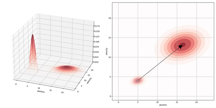
Since we converted our state space into the measurement space, we now have 2 comparable Gaussian PDFs:

• $μ{ₑₓₚ}$ and $Σ{ₑₓₚ}$ , which make up the Gaussian PDF for our predicted measurements
• $Z_{t}$ and $R_{t}$ , which make up the PDF for our sensor measurements

The strongest probability for our future state is the overlap between these two PDFs. How do we get this overlap?

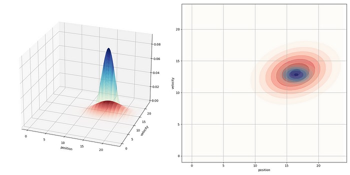
We multiply them together! The product of two Gaussian functions is just another Gaussian function. Even better, this common Gaussian has a smaller covariance than either the predicted PDF or the sensor PDF, meaning that our state is now much more certain.

ISN’T THAT NEAT.

Update Step, Solved.

We’re not out of the woods yet; we still need to derive the math! Suffice to say… it’s a lot. The basic gist is that multiplying two Gaussian functions results in its own Gaussian function. Let’s do this with two PDFs now, Gaussian functions with means μ₁, μ₂ and variances σ₁², σ₂². Multiplying these two PDFs leaves us with our final Gaussian PDF, and thus our final mean and covariance terms:

When we substitute in our derived state and covariance matrices, these equations represent the update step of a Kalman filter.

See reference (Bromiley, P.A.) for a good explanation on how >to multiply two PDFs and derive the above. It takes a good >page to write out; you’ve been warned.

This is admittedly pretty painful to read as-is. We can simplify this by defining the Kalman Gain $K_{t}$ :

With $K_{t}$ in the mix, we find that our equations are much kinder on the eyes:

We’ve done it! Combined, the new $X$ and P create our final Gaussian distribution, the one that crunches all of that data to give us our updated state. See how our updated state spikes in probability (the blue spike in Fig. 3). That’s the power of Kalman Filters!

What Now?

Well… do it again! The Kalman filter is recursive, meaning that it uses its output as the next input to the cycle. In other words, the final $X$ is your new $X_{t}$ ! The cycle continues in the next prediction state.

Kalman filters are great for all sorts of reasons:

• They extend to anything that can be modeled and measured. Automotives, touchscreens, econometrics, etc etc.
• Your sensor data can come from anywhere. As long as there’s a connection between state and measurement, new data can be folded in.
• Kalman filters also allow for the selective use of data. Did your sensor fail? Don’t count that sensor for this iteration! Easy.
• They are a good way to model prediction. After completing one pass of the prediction step, just do it again (and again, and again) for an easy temporal model.

Of course, if this is too much and you’d rather do… anything else, Tangram Vision is developing solutions to these very same problems! We’re creating tools that help any vision-enabled system operate to its best. If you like this article, you’ll love seeing what we’re up to.

Code Examples and Graphics

The code used to render these graphs and figures is hosted on Tangram Vision’s public repository for the blog. Head down, check it out, and play around with the math yourself! If you can improve on our implementations, even better; we might put it in here. And be sure to tweet at us with your improvements.

Check it out here:

Further Reading

If this article didn’t help, here are some other sources that dive into Kalman Filters in similar ways:

1. Faragher, R. (2012, September). Understanding the Basis of the Kalman Filter.
2. Bzarg. How a Kalman filter works, in pictures.
3. Teammco, R. Kalman Filter Simulation.
4. Bromiley, P.A. Products and Convolutions of Gaussian Probability Density Functions. [PDF]

Final note: Once again, this excellent tutorial was written by Tangram Vision CEO Brandon Minor