So you've learned some python. You built a cool little Todo App and a few Shopping Websites. But now it's time to take the next steps into the world of Computer Science, right?
Big-O may appear like a daunting thing to grasp at first but so was programming for everyone who first started. Let's see what Big-O is before we break it down.
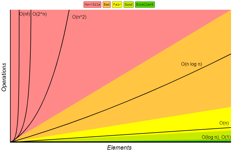
Image courtesy of BigOcheatsheets
Explain Big-O like I'm Five
In a direct to the point way, Big-O tells us how long an algorithm takes to run. Now I don't mean in seconds or milliseconds. I'm talking about how many iterations or operations it takes. What do I mean by this? let's look at a few examples.
Here we have a print method which in Big-O would be O(1)
def hello_world():
  print("Hello World!")

hello_world()
You can see in a simple print method it took us a single operation to print Hello World. If you see the chart above you can see O(1) is at the bottom representing it as the fastest method according to Big-O complexity. This is good right? Absolutely. Of course, nobody would pay us Devs to make Print statements all day.
Here is one more example of O(1)
def print_index_three(lists):
  print(lists[2])

# No matter how big our list, were still always calling index 3
print_index_three([1,2,3,4,5,6,7,8,9,10])
What about this next example? Were on the chart would you guess it fits?
my_list = ["Apple", "Mango", "Pear", "Cherry", "Grape", "Orange",
           "Blue Berry", "Papaya", "Melon", "Kiwi", "Banana"]

def find_fruit(lst, name)
  for fruit in lst:
    if fruit == name:
      return True

find_fruit(my_list, "Orange")
Our find_fruit function contains a for loop and an if statement. You might be thinking that's two operations, but in fact, it's still a single operation. Which in Big-O, is O(1)
Introducing a for loop is where our operations begin to go up.
As we can see my_list has 11 fruits. So our search function would pass over each element in the list 6 times to find Orange. Operations * 6.
or in Big-O: O(n)
What if the element we searched for was the first item on the list? Think about it, would it be O(1)? or O(n) still? It would be O(1) because it was a single operation to find the first element. This is called the best-case scenario in Big-O.
What about the worst-case scenario you might be wondering? Well, it would be the last element in my_list as it would take the most operations to complete our search function. Most of what makes Big-O theories are based on worst-case scenario.
When working with data, more often then not your software designs will have to keep scale in mind. Always ask yourself this question whenever possible.
"What is the worst-case scenario?"
A more efficient search algorithm
Our search function will do just fine with a few list items, but when we get a list of 100,000 items. We never know were in a list our target element is. To solve this, a common algorithm is a Binary Search.
def binary_search(lst, x):
    low = 0
    high = len(lst) - 1
    mid = 0

    while low <= high:

        mid = (high + low) // 2

        # Check if x is present at mid
        if lst[mid] < x:
            low = mid + 1

        # If x is greater, ignore left half
        elif lst[mid] > x:
            high = mid - 1

        # If x is smaller, ignore right half
        else:
            return mid

    # If we reach here, then the element was not present
    return -1

ordered_list = [1, 8, 13, 22, 31, 76, 79, 84, 92, 99]
#                             ^
#                       middle split

# Lets search for 79
print(binary_search(ordered_list, 79))
It's not very often that software engineers get to play with data that is sorted, but if you know it will be, binary search is the best choice for the question, What is the worst-case scenario?
A binary search falls under O(log n) on the Big-O complexity chart. If you already know what logarithms are, then I'm sure you can see why. Binary search will take the highest index of a list and split it right in the middle. Then run a O(1) operation where it checks if the element you're looking for is less than the current middle index. If it isn't it will ignore the left half, find a new middle index, and then repeat the process until it finds our elements index.
From the code example above, our target is 79. How many times would our algorithm iterate over splitting the list? It would take 3 operations. Giving us our log n If you decide to use a binary search in your near future, do keep in mind its effectiveness goes up, the more indices in a list.
Let's see a more Complex Example
Now if you're with me so far you can see the different Complexities of Big-O (O(n), O(1), O(log n))isn't too bad to understand. There simple math ideas representing how Complex an algorithm or function operates.
Let's see an actual Algorithm in action and show were on the Chart it belongs.
One of the first types of sort algorithm you will learn is a Merge-sort.
In a nutshell, it splits a list in half and then splits those lists in half repeatedly by calling itself Recursively and then compares them as it merges the list back up. See here or this video for more details.
If your not sure what Recursion is yet, see here.
def merge_sort(lst):
    if len(lst) >1:
        mid = len(lst) // 2 # The Middle of the list
        Left = lst[:mid]
        Right = lst[mid:]

        # As each list splits, you split those lists again. (Recursion)
        merge_sort(Left)
        merge_sort(Right)

        i = 0
        j = 0
        k = 0

        while i < len(Left) and j < len(Right):
            if Left[i] < Right[j]:
                lst[k] = Left[i]
                i += 1
            else:
                lst[k] = Right[j]
                j += 1
            k += 1

        # Check if any element was left.
        while i < len(Left):
            lst[k] = Left[i]
            i += 1
            k += 1

        while j < len(Right):
            lst[k] = Right[j]
            j += 1
            k += 1

my_list = [156, 42, 3, 78, 45, 22, 98, 100]

merge_sort(my_list)
print(my_list)
If this is your first time seeing a Merge-sort it might seem a bit complex but in fact, it isn't. In Big-O a Merge-sort falls under O(n log n ) which is pretty much in the middle of the time spectrum for how long the algorithm could take to finish.
What makes it O(n log n)? If we break down this expression in mathematical terms it is fairly easy to understand.
Operations * (elements log(elements))) In the example above we have 8 elements in the list. Which means that the list split in half 3 times. That is our log(n). After splitting 3 times we end up with 8 individual elements to compare with. That is our n

After all the elements are at their base(single item list) they then get sorted back up into 2 sorted lists(Left and Right). This now becomes the O(n) part of our O(n log n), Remember our example above using O(n)? The same thing is happening here except were comparing which number is the lowest. Then add it into the main sorted list we return.
The other half of the spectrum
There's a lot more too Big-O then I mentioned here. You have O(n^2), O(2^n), and even O(n!). But I wanted to keep this brief. I will be going over a lot more Big-O Complexities in the future as this is the first of many posts about Big-O.
Did you know that all Big-O Equations also have a Space Complexity too them also? You can actually find out how memory efficient your algorithms are too! If you're interested in Algorithms & Data Structures also, I will be posting about that too.
Additional resources worth checking out:
https://www.bigocheatsheet.com/

Top comments (2)
Great explanation!
I really like the visuals. Great post!