In this introductory post on Convolutional Neural Networks, we will cover:
- Some applications
- The most important layer types
While talking about the different layers, we won’t focus on the math but rather on the benefit of each layer as well as the simplified forward path.

Introduction to Convolutional Neural Networks (CNN)
Machine Learning offers many different models for supervised learning, and CNNs are one such model type. CNNs are part of the artificial neural network family, with the important addition that they contain convolutional layers. CNNs have many applications, such as image recognition and natural language processing. Let’s also mention that CNNs are inspired by the visual cortex of animals: neurons in the network only respond to the stimuli of a restricted region from the previous layer.
Why should you care about CNNs? Well a lot of the most challenging AI problems are actually solved with CNNs!😊
Applications
Let’s look at three innovative applications that work thanks to CNNs!
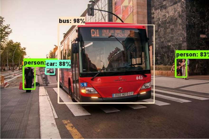
Object detection:
MobileNets, developed by Google Research, can be used for many tasks, among them object detection. The advantage of MobileNets: this neural network family is very resource efficient, which can be crucial for applications running on smartphones or autonomous cars.
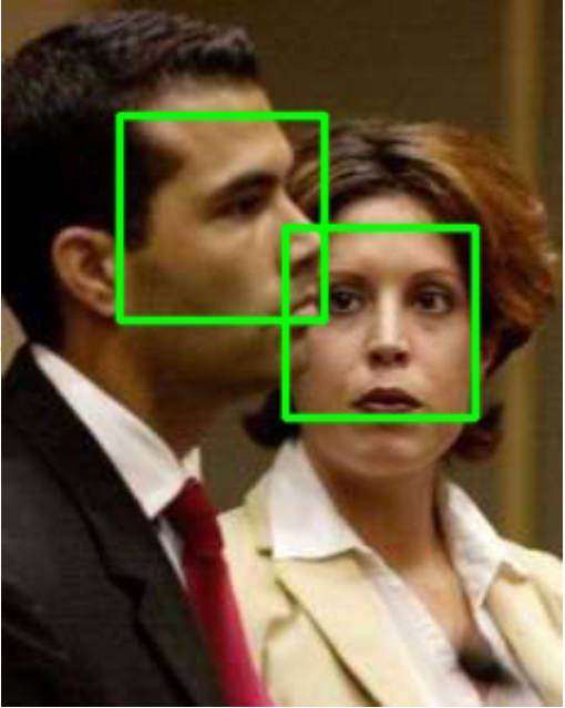
Face recognition:
Stevens Institute of Technology used CNNs for face detection, one possible application: focus smartphone camera on the people, not the background.
Board game Go:
DeepMind used a combination of deep neural network and tree search to beat the best human player at the game of Go.

The layers
Convolutional neural networks typically contain many layers – some models up to 100 layers and more! Each layer is supposed to extract features – that is, interesting characteristics – from the input. Since CNNs often consist of so many layers, they are part of the deep learning models.
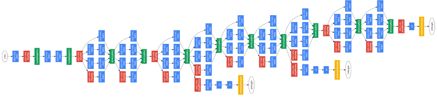
Image credit: Google Research
Above, you can see the picture of a deep CNN called GoogleNet. As the name suggests, it was designed by Google. On the very left of the picture, the input (that is, an image in RGB format) is fed into the CNN. The first layers extract very simple features like lines, dots and edges in the image. The next layers extract more advanced features like objects and shapes. At the very right of the picture above, the network will extract high level features which enable to the network to distinguish between 1000 image categories.
You might ask: So which layers exist and when should I use them? Well I’m glad you asked: This blog will answer exactly this question! 😊 First let’s get an overlook of the most important layer types:
| Layer type | Benefit | Has learnable parameters? |
|---|---|---|
| Convolution | Extract feature from small region of input | Yes |
| Fully connected | Extract feature from whole input | Yes |
| ReLU | Recognize non-linear properties | No |
| Pooling | Resilient against small distortion in input | No |
| Batch Normalization | Keep neuron values in range | Yes |
| Softmax | Get class probabilities | No |
| Loss | Calculate the prediction error | No |
Now let’s go through all layer types:
Convolutional layer
Convolutional layers are typically where most of the computation happens in a deep CNN: this layer type extracts features using a K x K convolution filters. An example is given below, where the green input is convolved with the yellow filter and thus the red output is generated. In this example, the filter dimension K equals 3. The output shows high values in spatial locations where the input looks similar to the filter.
Image credit: Stanford Tutorial
As you can see, we extract the same feature at different spatial locations. This means the output only depends on a small region of the input.
In reality, things are slightly more complicated than in the image above: the input to a convolutional layer consists of multiple feature maps, and the output too. So, for N input feature maps and M output feature maps, we need filters in the total size of N * M * K * K.
Convolutional layers are typically the bottle neck in terms of arithmetic operations. In most deep learning frameworks, convolution is implemented via data rearranging and matrix multiplication. Also, deep learning training is very resource intense, but offers a lot of room for parallelism. For this purpose, people often use Graphics Processing Units for training, and matrix multiplications are heavily optimized on modern GPUs.
For a great way to learn more about convolution, you can check this course offered by Stanford University. They also cover more details on CNNs in general.
Fully Connected Layer
Alright, let’s move on to the next layer type, namely the fully connected layer. This layer extracts features over the whole input, meaning each output node depends on all input nodes. Mathematically, the output vector y is the result of the weighted input vector x:
y = W * x
The weight matrix W is of dimension |x|*|y|, which brings us to the drawback of this layer type: The size of the parameters tends to be very large, which is why most modern network architectures avoid fully connected layers.
Activation Function: ReLU
Convolutional neural networks can capture complex properties, which wouldn’t be recognized by a simple linear regression. This is largely thanks to activation functions inside a neural network: They introduce a non-linearity into the forward path of the network. Activation functions are typically appended to the convolutional layers and they are applied to each output node independently.
Traditionally, people used different activation functions like Sigmoid, Tanh and ReLU. The last one has proven to be the most effective for deep learning. The picture below shows all three activation functions:
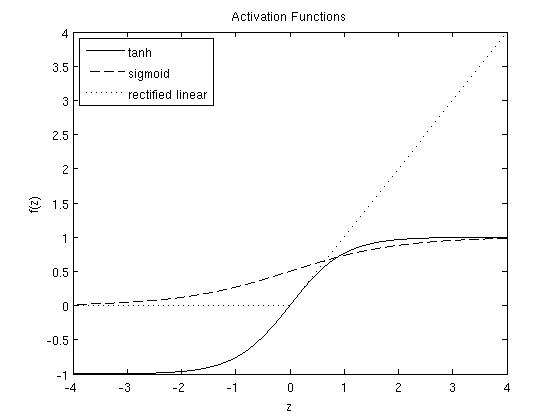
The activation function ReLU (Rectified Linear Unit) keeps all positive values untouched, but negative values get set to zero:
y = max(0, x)
Pooling Layer
Pooling layers reduce the dimension by combining several neurons to one. There are two pooling types: average pooling and max pooling. Many networks use max pooling: here, the output node is equal to the maximum of the input region.
Image credit: Stanford Tutorial
Batch Normalization
For different reasons which we’ll discuss in a second, we want our activations to stay in a reasonable number range during training. However, the above presented ReLU activation function is unbounded. To make up for this, we typically use normalization layers at regular intervals within the network. There are two important normalization layer types: LRN (local response normalization) and BN (batch normalization). While older networks used LRN, newer ones often use BN. BN was originally proposed by Google Research and it helps in many ways: the training is easier to set up and goes faster, and the end accuracy is better. What BN basically does, is it rescales and re-centers the data.
So why is it important to keep our data in a reasonable range? There are two main reasons: First we need to represent our data using some number format (typically with 32-bit or 64-bit floating point), and we simply can’t represent huge numbers accurately. Second, we want high values in our feature maps to represent strong feature existence. But values down the layer chain would possibly become huge, thus we can’t easily estimate whether a given feature is actually present or not.
Once the network is trained and then used for inference, the BN layer can be simplified to a linear transformation:
y = γ * x + β
Softmax
The output of a classification network is a vector of probabilities. To achieve this, we use a Softmax layer, which normalizes the output nodes such that the sum of all nodes is 1. The formula of Softmax is as follows:
y = exp(x) / sum(exp(x))
Loss
The loss layer is used during training only. It compares the network output with the ground truth and computes the “error” of our prediction. The resulting loss is then backpropagated through the network to adjust all learnable parameters. Various loss functions exist, and the choice of loss function will often influence the final result significantly.
For multi-class prediction networks, we typically use Sparse Cross Entropy as loss function, which is equal to the negative log probability of the true class. If our network is sure of the correct class, the loss is zero, and if the network is totally wrong, the loss is infinitely big.
Conclusion
In this post, we first covered the benefits of neural networks: for tasks like object detection, they deliver state-of-the-art results. The second part of the blog was dedicated to the different layer types which are commonly used in CNNs. If you wish to dive deeper and gain more hands-on experience with CNNs, I can suggest this TensorFlow CNN Tutorial.
Thanks so much for reading this blog, I hope it has helped you to get started with CNNs.😊

Top comments (0)