
Gradient Descent in Linear Regression
Gradient Descent is a first order optimization algorithm to find the minimum of a function.It finds the minimum (local) of a function by moving along the direction of steep descent (downwards). This helps us to update the parameters of the model (weights and bias) more accurately.
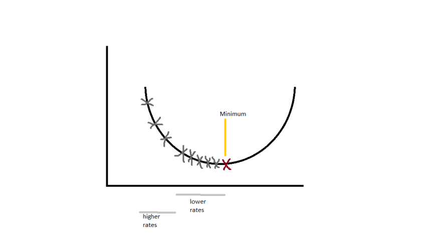
To get to the local minima we can't just go directly to the point (on a graph plot). We need to descend in smaller steps and check for minima and take another step to the direction of descent until we get our desired local minimum.
The small steps mentioned above is called as learning rate. If the learning rate is very small the precision is more but is very time consuming. And large learning rate may lead us to miss the minimum (overshooting). The theory is to use the learning rate at higher rate until the slope of curve starts to decrease ad once it starts decreasing, we start using smaller learning rates(Less time and More Precision).
The cost function helps us to evaluate how good our model is functioning or predicting. Its a loss function. It has its own curve and parameters (weights and bias). The slope of the curve helps us to update our parameters accordingly. The less the cost more the predicted probability.
In the training phase, we are finding the y_train value to find how much is the value is deviating from the given output. Then we calculate the cost error in the given second phase by using the cost error formula.
y_train = w * xi + b
cost = (1/N) * ∑(yi − y_train)2 {i from 1 to n}
for i in range(n_iters):
    #Training phase
    y_train = np.dot(X, self.weights) + self.bias

    #Cost error calculating Phase
    cost = (1 / n_samples) * np.sum((y_train - y)**2)
    costs.append(cost)
Now we update the weights and bias to decrease our error by doing
    #Updating the weight and bias derivatives
    Delta_w = (2 / n_samples) * np.dot(X.T, (y_hat - y))
    Delta_b = (2 / n_samples) * np.sum((y_hat - y))

    #Updating weights
    self.weights = self.weights - learn_rate * Delta_w
    self.bias = self.bias - learn_rate * Delta_b

    # end of loop
And ploting cost function against iterations

Above given is a cost function curve against number of iterations. As number of iterations increases (steps) cost decreased drastically meaning minimum is nearby and almost became zero. We do the above updations until the error becomes negligible or minimum is reached.
Source code from Scratch
class LinearModel:
    """
    Linear Regression Model Class
    """
    def __init__(self):
        pass

    def gradient_descent(self, X, y, learn_rate=0.01, n_iters=100):
        """
        Trains a linear regression model using gradient descent
        """
        n_samples, n_features = X.shape
        self.weights = np.zeros(shape=(n_features,1))
        self.bias = 0
        self.prev_weights = []
        self.prev_bias = []
        self.X = X
        self.y = y
        costs = []

        for i in range(n_iters):
            """"
            Training Phase
            """
            y_hat = np.dot(X, self.weights) + self.bias
            """
            Cost error Phase
            """
            cost = (1 / n_samples) * np.sum((y_hat - y)**2)
            costs.append(cost)
            """
            Verbose: Description of cost at each iteration
            """
            if i % 200 == 0:
                print("Cost at iteration {0}: {1}".format(i,cost))
            """
            Updating the derivative
            """
            Delta_w = (2 / n_samples) * np.dot(X.T, (y_hat - y))
            Delta_b = (2 / n_samples) * np.sum((y_hat - y))

            """"
            Updating weights and bias
            """
            self.weights = self.weights - learn_rate * Delta_w
            self.bias = self.bias - learn_rate * Delta_b

            """
            Save the weights for visualisation
            """
            self.prev_weights.append(self.weights)
            self.prev_bias.append(self.bias)

        return self.weights, self.bias, costs

    def predict(self, X):
        """
        Predicting the values by using Linear Model
        """
        return np.dot(X, self.weights) + self.bias
# We have created our Linear Model class. Now we need to create and load our model.
model = LinearModel()

w_trained, b_trained, costs = model.gradient_descent(X_train, y_train, learn_rate=0.005, n_iters=1000)

    def visualize_training(self):
        """
        Visualizing the line against the dataset
        """

        self.prev_weights = np.array(self.prev_weights)

        x = self.X[:, 0]
        line, = ax.plot(x, x, color='red')
        ax.scatter(x, self.y)


        def animate(line_data):
            m, c = line_data
            line.set_ydata(m*x + c)  # update the data
            return line,

        def init():
            return line,

        def get_next_weight_and_bias():
            for i in range(len(self.prev_weights)):
                yield self.prev_weights[i][0], self.prev_bias[i]

        return animation.FuncAnimation(fig, animate, get_next_weight_and_bias, init_func=init,interval=35, blit=True)
# Visualization of training phase to get the best fit line
fig, ax = plt.subplots()
ani = model.visualize_training()
plt.show()

# Prediction Phase to test our model
n_samples, _= X_train.shape
n_samples_test, _ = X_test.shape

y_p_train = model.predict(X_train)
y_p_test = model.predict(X_test)

error_train =  (1 / n_samples) * np.sum((y_p_train - y_train) ** 2)
error_test  =  (1 / n_samples_test) * np.sum((y_p_test - y_test) ** 2)

print("Error on training set: {}".format(np.round(error_train, 6)))
print("Error on test set: {}".format(np.round(error_test, 6)))

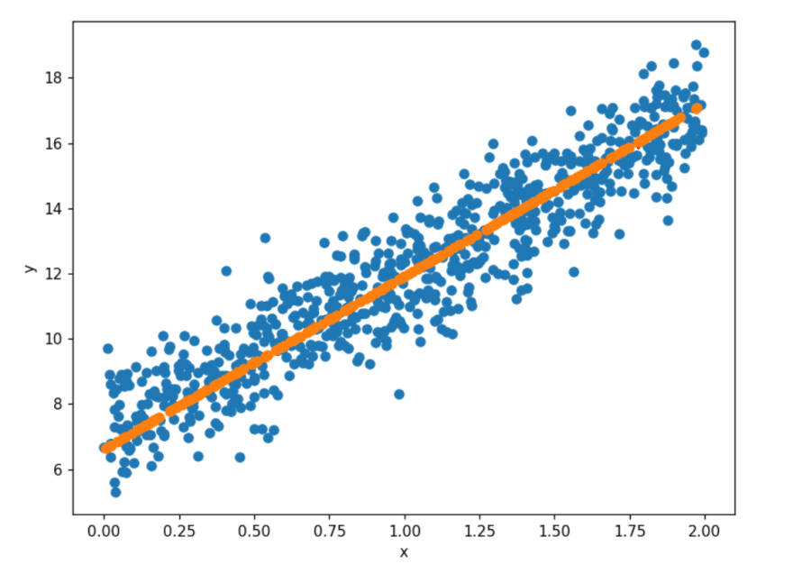
# Plotting predicted best fit line
fig = plt.figure(figsize=(8,6))
plt.scatter(X_train, y_train)
plt.scatter(X_test, y_p_test)
plt.xlabel("x")
plt.ylabel("y")
plt.show()
Check out the full source code for Gradient Descent on GitHub
and also check out the other approaches in Linear Regression by ML-Scratch
Contributors
This series is made possible by help from:
- Pranav (@devarakondapranav )
- Ram (@r0mflip )
- Devika (@devikamadupu1 )
- Pratyusha(@prathyushakallepu )
- Pranay (@pranay9866 )
- Subhasri (@subhasrir )
- Laxman (@lmn )
- Vaishnavi(@vaishnavipulluri )
- Suraj (@suraj47 )

Top comments (0)