
The idea behind simple linear regression is to "fit" the observations of two variables into a linear relationship between them. Graphically, the task is to draw the line that is "best-fitting" or "closest" to the points.
The equation of a straight line is written using the y = mx + b, where m is the slope (Gradient) and b is y-intercept (where the line crosses the Y axis).Where, m is the slope (Gradient) and b is y-intercept (Bias).In calculation of mean and y-intercept, we use some of the mathematical concepts explained below:
Mean
This term is used to describe properties of statistical distributions. It is determined by adding all the data points in a population and then dividing the total by the number of points. The resulting number is known as the mean or the average.
x̄ = Sum of observations / number of observationsVariance
Variance (σ2) is a measurement of the spread between numbers in a data set. That is, it measures how far each number in the set is from the mean and therefore from every other number in the set.
Variance = n * sum of all(xi − x̄)2
Where:
xi = ith data point
x̄ = the mean of all data points
n = the number of data points
Co-variance
Covariance is a measure of how much two random variables vary together. It’s similar to variance, but where variance tells you how a single variable varies, co-variance tells you how two variables vary together.Square root of variance is called Standard Deviation
Cov(X,Y) = Σ (E(X) - μ) * (E(Y) - ν) / (n - 1) Where
X is a random variableE(X) = μ is the expected value (the mean) of the random variable XE(Y) = ν is the expected value (the mean) of the random variable Yn = the number of items in the data set
Correlation
Correlation(r) is a statistical technique that can show whether and how strongly pairs of variables are related.
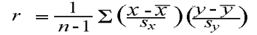
Sx, Sy = Standard deviation of x, yRoot Mean Square Error (RMSE)
Root Mean Square Error (RMSE) is the standard deviation of the residuals(prediction errors). Residuals are a measure of how far from the regression line data points are.

Calculation of Slope and Bias
The slope of the line is calculated as the change in y divided by change in x.
slope m = change in y / change in xThe y-intercept over bias shall be calculated using the formula
y = m(x - x1) + y1These values are different from what was actually there in the training set and if we plot this (x, y) graph against the original graph, the straight line will be way off the original points in the graph. This may lead to error which is the difference of values between actual points and the points on the straight line. Ideally, we’d like to have a straight line where the error is minimized across all points.Error can be reduced using many mathematical ways. One of such method is "Least Square Regression"
Least Square Regression
Least Square Regression is a method which minimizes the error in such a way that the sum of all square error is minimized.
m = (Σ ((x - x̄) * (y - ȳ)) / Σ (x - x̄))2(or)
m = r(Sy / Sx)(and we get the y-interept)
b = ȳ - m * x̄Where
Sx is standard deviation of x
Sy is standard deviation of y
r is correlation between x and y
m is slope
b is the y-intercept
This method is intended to reduce the sum square of all error values. The lower the error, lesser the overall deviation from the original point.
Cost Function
The cost function calculates the square of the error for each example in the dataset, sums it up and divides this value by the number of examples in the dataset (denoted by m).This cost function helps in determining the best fit line.The cost function for two variables θ0 and θ1 denoted by J and is given as follows.
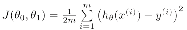
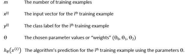
Now, we have to make use of cost function to adjust our parameters θ0 and θ1 such that they result in the least cost function value. We make use of a technique called Gradient Descent to minimize the cost function.
Read On 📝
Contributors
This series is made possible by help from:
- Pranav (@devarakondapranav )
- Ram (@r0mflip )
- Devika (@devikamadupu1 )
- Pratyusha(@prathyushakallepu )
- Pranay (@pranay9866 )
- Subhasri (@subhasrir )
- Laxman (@lmn )
- Vaishnavi(@vaishnavipulluri )
- Suraj (@suraj47 )

Top comments (0)