Progressive Growing GANs for Improved quality PGGAN
What's PGGAN? Progressive Growing of GANs for Improved Quality, Stability, and Variation. Key idea is to grow both the generator and discriminator progressively. Starting from a low resolution, I add new layers that model increasingly fine details as training progresses. This both speeds the training up and greatly stabilizes it, allowing us to produce images of unprecedented quality, e.g., CelebA images at 1024^2. Also propose a simple way to increase the variation in generated images, and achieve a record inception score of 8.80 in unsupervised CIFAR10. Additionally, describe several implementation details that are important for discouraging unhealthy competition between the generator and discriminator. Finally, I suggest a new metric for evaluating GAN results, both in terms of image quality and variation. As an additional contribution, I could construct a higher-quality version of the CelebA dataset.
Figures
Progressive growing of GANs

Train starts with both the generator G and discriminator D having a low spatial resolution of 4X4 pixels. As advances, I add layers to G and D for spatial resolution of the generated images. All layers remain trainable throughout the process. NXN refers to convolutional layers operating on NXN spatial resolution. This allows stable synthesis in high resolutions and also speeds up training considerably. One the right, six pictures above generated using progressive growing at 1024X1024.
- 생성기와 분류기의 layer를 대칭적으로 하나씩 쌓아가며 학습할 경우 Large scale structure 먼저 파악한 후 세세한 Finer scale details로 좁혀가는 원리이다. Layer를 늘리는 시점의 충격을 완화하기 위해 Highway Network의 구조를 사용하여 학습의 안정성과 속도를 올릴 수 있다.
Highway Network

When doubling the resolution of generator G and discriminator D I fade in the new layers smoothly. This illustrates the transition from 16X16 images to 32X32 images.
During the transition b, the layers that operate on the higher resolution like a residual block, whose weight increases linearly from 0 to 1. toRGB a layer that projects feature vectors to RGB colors and fromRGB does the reverse both 1X1 convolutions. When training the discriminator, real images that are downscaled to match the current resolution of the network. During a resolution transition, interpolate between two resolutions of the real images, similarly to how the generator output combines two resolutions.
def lerp(a, b, t): return a + (b - a) * t
def lerp_clip(a, b, t): return a + (b - a) * tf.clip_by_value(t, 0.0,           1.0)
//omitted
if structure == 'linear':
img = images_in
x = fromrgb(img, resolution_log2)
for res in range(resolution_log2, 2, -1):
    lod = resolution_log2 - res # lod: levels-of-details
    x = block(x, res)
    img = downscale2d(img)
    y = fromrgb(img, res - 1)
    with tf.variable_scope('Grow_lod%d' % lod):
        x = lerp_clip(x, y, lod_in - lod)
- 비지도학습 GAN은 학습 데이터의 variation에 대한 subset만을 학습하는 경향이 있다. Minibatch Discriminator 라는 기법을 통해 각 이미지와 미니배치의 정보를 분류기에 같이 제공함으로써 다양성에 대한 학습 효과를 증진시키고 새로운 파라미터 없이 진행을 한다.
- 전체 minibatch에 대해, 각 feature의 각 spatial location의 표준편차를 구한다. (Input: N x Cx H x W, Output: C x H x W)
- 앞서 계산된 값으로 각 spatial location에서 모든 feature에 대한 평균을 구한다. (Input: C x H x W, Output: 1 x H x W)
- 계산된 평균을 마지막 샘플 layer 뒤에 추가한다.

Normalization in gerator and discriminator
-
Equalized learning rate: 기존 방식과 달리 weight의 초기화는 N(0,1)로 하되, runtime 중에 동적으로 weight parameter의 스케일을 조절해주자는 아이디어. He initializer에서 제안된 per-layer normalization constant로 weight parameter를 나누어준다. 사람들에게 즐겨 사용되는 RMSProp이나 ADAM의 경우 gradient update에 대해 normalizing을 해주게 되는데, 이것이 parameter들에 대한 scale과는 별개로 계산되는 것이기 때문에 변동이 큰 parameter에 대해서는 학습에 효과적이지 않을 수 있다. 이 방법을 사용하면 모든 parameter가 같은 dynamic range를 갖게 하므로 동일한 학습속도를 보장할 수 있다.
def get_weight(shape, gain=np.sqrt(2), use_wscale=False, fan_in=None):
if fan_in is None: fan_in = np.prod(shape[:-1])
std = gain / np.sqrt(fan_in)
if use_wscale:
    wscale = tf.constant(np.float32(std), name='wscale')
    return tf.get_variable('weight', shape=shape, initializer=tf.initializers.random_normal())
else:
    return tf.get_variable('weight', shape=shape, initializer=tf.initializers.random_normal(0, std))
✔️ GAN은 generator와 discriminator간의 unhealthy competition으로 인해 signal magnitude가 점차 증가되기 쉽다. 이에 대한 해결책으로 이전의 연구들에서 변형된 batch normalization의 사용이 제안되었으나, GAN에서는 이슈는 (BN에서 제기된 문제상황이었던) covariate shift가 아니므로 이 연구에서는 signal magnitude와 competition에 대해 적절히 제한하는 것에 초점을 맞춘다.
✔️ Pixelwise feature vector normalization in generator: generator와 discriminator의 magnitude가 competition에 의해 통제불능의 상태가 되는 것을 막기위해 각 convolutional layer의 feature layer에 대해 pixel 단위로 normalizing을 해준다. 결과물의 품질에 큰 영향을 준 것은 아니지만 필요시 signal magnitudes가 점차 증가되는 것을 막아주었다.
def pixel_norm(x, epsilon=1e-8):
with tf.variable_scope('PixelNorm'):
    return x * tf.rsqrt(tf.reduce_mean(tf.square(x), axis=1, keepdims=True) + epsilon)
Increasing Variation using MiniBatch Standard Deviation
현재 해상도에 맞춰 우리가 가지고 있는 Real Images를 Downscaling 하면 저해상도 이미지도 바뀌게 된다. 하지만 고해상도 이미지에 대한 정보도 담고 있다는 것을 알아두자. 두개의 해상도 사이를 선형보간 (interpolation)하는 과정을 거치며 학습을 진행한다. 일반적인 비지도학습의 특징으로 훈련 중 train data에서 찾은 feature information보다 less variation한 generator image를 생성해내는 경향이 있다. 그로 인한 고해상도 이미지를 생성해내기 어렵다는 단점이 발생하게 되는데 이를 해결하고자 PGGAN 에서는 표준편차 미니배치 기법을 제안한 것이다. 이를 사용하면 Discriminator 가 미니배치 전체에 대한 Feature statistics 를 계산하도록 하기 위해서 실제 훈련 데이터와 Fake batch 이미지를 구별해내도록 도움을 줄 수 있다. 또한 생성된 배치 이미지에서 계산된 Feature statics가 training된 batch image data의 Statics와 더 유사하게 만들도록 생성기가 낮은 분산값을 갖는게 아닌 더 풍부한 분산값을 갖도록 권장한다!
Convergence and Training Speed

High-Resolution Image Generation Using CELEBA-HQ Datasets

- 고해상도 결과를 위해서는 8 Telsa V100 GPU로 4일간의 훈련이 필요하다.
Conclusion
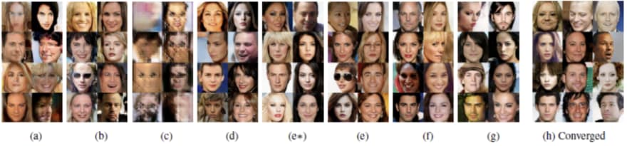
- MS-SSIM에 비해 SWD가 색, 질감, 뷰포인트에 대한 variation을 훨씬 잘 잡아냄. 학습이 중간에 중단된 모델과 학습을 온전히 끝낸 모델간의 결과물을 비교했을때 MS-SSIM는 큰 차이를 잡아내지 못했다. 또한 SWD는 training set과 유사한 생성 이미지의 분포에 대해 잘 찾아내는 모습을 보였다.
- progressive growing은 better optimum에 수렴시키고 training time을 줄이는 효과를 보였다. 약 640만개의 이미지 학습을 기준으로 non-progressive variant에 비해 약 5.4배 빠른 속도를 보였다.
- High resolution output을 보이기 위해 AppendixC의 방법을 사용해 CELEBA의 high-quality 버전을 만들어냈다. (1024 x 1024, 30000 장) Tesla V100 GPU 8개로 4일동안 학습하였고 아주 멋진 결과물을 만들어냈다. (위에 데모 참고)학습에는 LSGAN과 WGAN-GP의 loss function이 각각 사용되었는데, 아무래도 LSGAN이 학습에 좀 더 불안정한 모습을 보였다. LSGAN의 loss function을 사용하는 경우에는 약간의 추가적인 테크닉이 필요한데, 이는 Appendix B를 참고하자.


Top comments (0)