PostgreSQL has several built-in window functions, and they provide the ability to perform calculations across rows related to the current query row. In the previous article, I laid out the basic concept of how window functions work. In this article, I will give an overview of a handful of these window functions. The windows functions are split into four categories: aggregate, ranking, distribution, and analytic functions.
The built-in window functions are listed below.
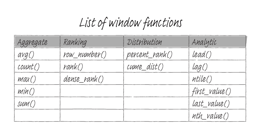
Except for functions in the aggregate column, all other functions require an OVER clause to work.
Aggregate window functions
One use case for a window function is to calculate moving average and moving total. We can achieve this using aggregate functions. Remember that aggregate functions act as window functions only when there is an OVER clause after the function. If you omit the OVER clause, they work like ordinary aggregates and return a single row for the entire set. You can use all built-in plain aggregate functions as a window function. But in this article, I only use five of them.
| Functions | What it does |
|---|---|
| AVG(args) | Average (arithmetic mean) of all the non-null input values within a window frame. |
| COUNT(args) | Count of non-null values within a window frame. |
| MAX(args) | Maximum value of the non-null values within a window frame. |
| MIN(args) | Minimum value of the non-null values within a window frame. |
| SUM(args) | Sum of non-null values within a window frame. |
Aggregate functions do not require an ORDER BY, but they accept window frame definition (ROWS, RANGE, and GROUPS).
The following query shows the aggregate functions in action.
SELECT customer_id AS cid,
       billing_city AS city,
       total,
       ROUND(AVG(total) OVER(PARTITION BY billing_city), 2) AS avg,
       COUNT(total) OVER(PARTITION BY billing_city) AS count,
       MAX(total) OVER(PARTITION BY billing_city) AS max,
       MIN(total) OVER(PARTITION BY billing_city) AS min,
       SUM(total) OVER(PARTITION BY billing_city) AS sum
FROM invoice;
 cid |   city    | total | avg  | count |  max  | min  |  sum
-----+-----------+-------+------+-------+-------+------+-------
  48 | Amsterdam |  1.98 | 5.80 |     7 | 13.86 | 0.99 | 40.62
  48 | Amsterdam | 13.86 | 5.80 |     7 | 13.86 | 0.99 | 40.62
  48 | Amsterdam |  0.99 | 5.80 |     7 | 13.86 | 0.99 | 40.62
  48 | Amsterdam |  8.91 | 5.80 |     7 | 13.86 | 0.99 | 40.62
  48 | Amsterdam |  8.94 | 5.80 |     7 | 13.86 | 0.99 | 40.62
  48 | Amsterdam |  3.96 | 5.80 |     7 | 13.86 | 0.99 | 40.62
  48 | Amsterdam |  1.98 | 5.80 |     7 | 13.86 | 0.99 | 40.62
  59 | Bangalore |  1.99 | 6.11 |     6 | 13.86 | 1.98 | 36.64
  59 | Bangalore |  8.91 | 6.11 |     6 | 13.86 | 1.98 | 36.64
  59 | Bangalore |  1.98 | 6.11 |     6 | 13.86 | 1.98 | 36.64
  59 | Bangalore | 13.86 | 6.11 |     6 | 13.86 | 1.98 | 36.64
  59 | Bangalore |  3.96 | 6.11 |     6 | 13.86 | 1.98 | 36.64
  59 | Bangalore |  5.94 | 6.11 |     6 | 13.86 | 1.98 | 36.64
 <------------------------ TRUNCATED ------------------------->
Ranking functions
Another use case for using the window function is assigning an ordinal number to rows, and PostgreSQL provides three functions to handle this.
| Functions | What it does |
|---|---|
| ROW_NUMBER() | Returns the number of the current row within a window partition. The numbers are unique. |
| RANK() | Returns the rank of the current row within a partition. There will be gaps and tied values. |
| DENSE_RANK() | Returns the rank of the current row within a partition, without gaps, but there will be tied values. Think of it as counts for peer groups. |
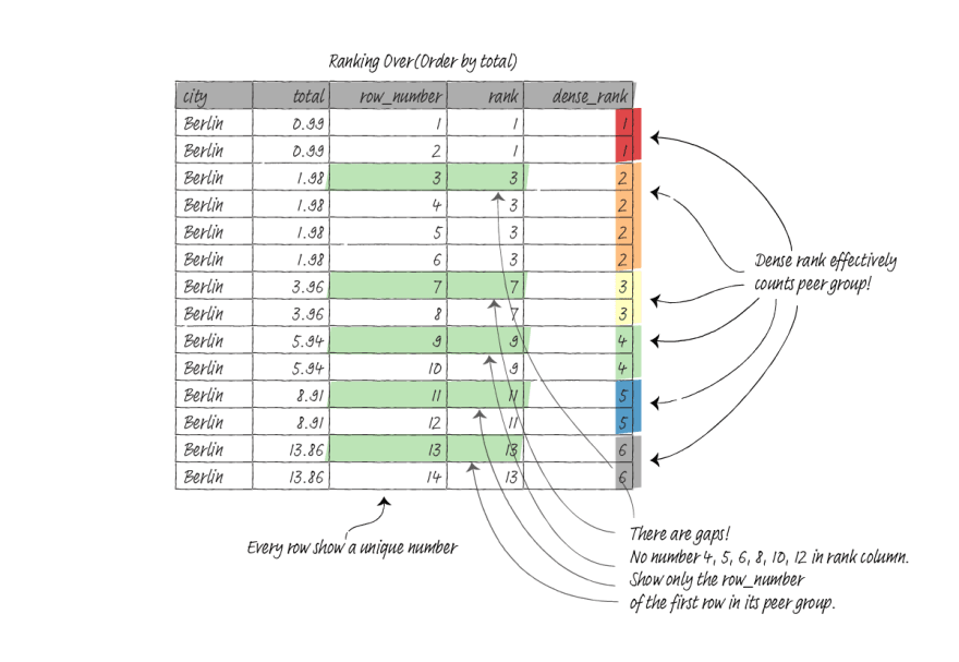
ROW_NUMBER() does not require ORDER BY, but RANK() and DENSE_RANK() require ORDER BY to work. None of these functions accept window frame definitions.
The following query show ROW_NUMBER(), RANK(), DENSE_RANK() in action.
SELECT customer_id AS cid,
       billing_city AS city,
       total,
       ROW_NUMBER() OVER(PARTITION BY billing_city) AS row_number,
       RANK() OVER(PARTITION BY billing_city ORDER BY total) AS rank,
       DENSE_RANK() OVER(PARTITION BY billing_city ORDER BY total) AS dense_rank
FROM invoice;
 cid | city         | total | row_number | rank | dense_rank
-----+--------------+-------+------------+------+------------
  48 | Amsterdam    |  0.99 |          1 |    1 |          1
  48 | Amsterdam    |  1.98 |          2 |    2 |          2
  48 | Amsterdam    |  1.98 |          3 |    2 |          2
  48 | Amsterdam    |  3.96 |          4 |    4 |          3
  48 | Amsterdam    |  8.91 |          5 |    5 |          4
  48 | Amsterdam    |  8.94 |          6 |    6 |          5
  48 | Amsterdam    | 13.86 |          7 |    7 |          6
  59 | Bangalore    |  1.98 |          1 |    1 |          1
  59 | Bangalore    |  1.99 |          2 |    2 |          2
  59 | Bangalore    |  3.96 |          3 |    3 |          3
  59 | Bangalore    |  5.94 |          4 |    4 |          4
  59 | Bangalore    |  8.91 |          5 |    5 |          5
  59 | Bangalore    | 13.86 |          6 |    6 |          6
 <------------------------ TRUNCATED ------------------------->
Distribution functions
Distribution functions require ORDER BY, and they do not accept window frame definitions.
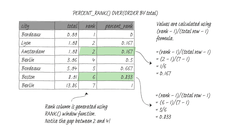
Percent rank
PERCENT_RANK() returns the relative rank of the current row. It is calculated using a simple formula: (rank - 1) / (total partition rows - 1). The value ranges from 0 to 1 inclusive.
The following query shows PERCENT_RANK() in action. In this particular example, I also partition the data according to the billing city.
SELECT customer_id AS cid,
       billing_city AS city,
       total,
       PERCENT_RANK() over(PARTITION BY billing_city ORDER BY total)
FROM invoice;
   city        | total |    percent_rank
--------------------+-------+---------------------
 Amsterdam     |  0.99 |                   0
 Amsterdam     |  1.98 | 0.16666666666666666
 Amsterdam     |  1.98 | 0.16666666666666666
 Amsterdam     |  3.96 |                 0.5
 Amsterdam     |  8.91 |  0.6666666666666666
 Amsterdam     |  8.94 |  0.8333333333333334
 Amsterdam     | 13.86 |                   1
 Bangalore     |  1.98 |                   0
 Bangalore     |  1.99 |                 0.2
 Bangalore     |  3.96 |                 0.4
 Bangalore     |  5.94 |                 0.6
 Bangalore     |  8.91 |                 0.8
 Bangalore     | 13.86 |                   1
<---------------- TRUNCATED ---------------->
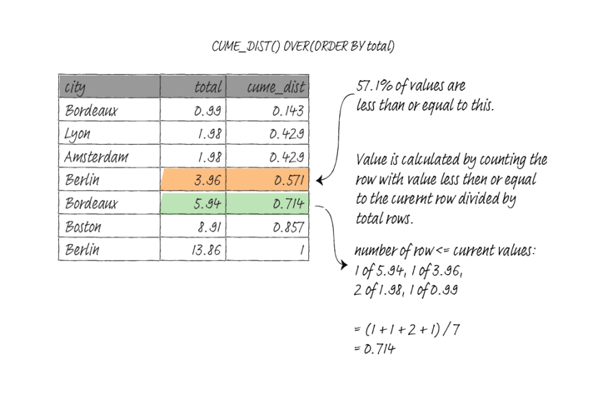
Cumulative distribution
CUME_DIST() returns the cumulative distribution within a group of values. The value range from 1/N to 1, and you calculate this by dividing the number of rows with values less than or equal to the current row's value to the total number of rows.
The following query show CUME_DIST() in action.
SELECT billing_city as city,
       total,
       CUME_DIST() over(PARTITION BY billing_city ORDER BY total)
FROM invoice;
PARTITION BY is not mandatory for CUME_DIST, but I used it to show cumulative distribution within a city in this example.
       city         | total |      cume_dist
--------------------------+-------+---------------------
 Amsterdam           |  0.99 | 0.14285714285714285
 Amsterdam           |  1.98 | 0.42857142857142855
 Amsterdam           |  1.98 | 0.42857142857142855
 Amsterdam           |  3.96 |  0.5714285714285714
 Amsterdam           |  8.91 |  0.7142857142857143
 Amsterdam           |  8.94 |  0.8571428571428571
 Amsterdam           | 13.86 |                   1
 Bangalore           |  1.98 | 0.16666666666666666
 Bangalore           |  1.99 |  0.3333333333333333
 Bangalore           |  3.96 |                 0.5
 Bangalore           |  5.94 |  0.6666666666666666
 Bangalore           |  8.91 |  0.8333333333333334
 Bangalore           | 13.86 |                   1
Analytic functions
Lead and lag
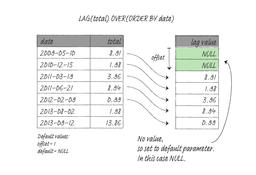
LEAD(args, offset, default) returns a value that comes after the current row by an offset. If there is no row after the offset, it will return default. If you don't specify, the offset value will be one, and the default will be NULL.

LAG(args, offset, default) returns a value that comes before the current row by an offset. If there is no row before the offset, it will return default. If you don't specify, the offset value will be one, and the default will be NULL.
The default value for both functions must be of a type that is compatible with the row value. So you might need to cast it or use :: operator to match the column data type.
Both LEAD and LAG require an ORDER BY clause, but they do not accept window frame definition.
The following query shows LEAD() and LAG() in action. Notice to set the default to 0, and I must cast the data type to match the total column data type, which is numeric.
SELECT billing_city AS city,
       invoice_date::DATE as date,
       total,
       LEAD(total) OVER(
           PARTITION BY billing_city
           ORDER BY invoice_date
       ) as lead,
       LAG(total, 2, 0::numeric) OVER(
           PARTITION BY billing_city
           ORDER BY invoice_date
           RANGE BETWEEN UNBOUNDED PRECEDING
              AND UNBOUNDED FOLLOWING
       ) as lag
FROM invoice;
 city         |    date    | total | lead  |  lag
-------------------+------------+-------+-------+-------
 Amsterdam    | 2009-05-10 |  8.91 |  1.98 |     0
 Amsterdam    | 2010-12-15 |  1.98 |  3.96 |     0
 Amsterdam    | 2011-03-19 |  3.96 |  8.94 |  8.91
 Amsterdam    | 2011-06-21 |  8.94 |  0.99 |  1.98
 Amsterdam    | 2012-02-09 |  0.99 |  1.98 |  3.96
 Amsterdam    | 2013-08-02 |  1.98 | 13.86 |  8.94
 Amsterdam    | 2013-09-12 | 13.86 |       |  0.99
 Bangalore    | 2009-04-05 |  3.96 |  5.94 |     0
 Bangalore    | 2009-07-08 |  5.94 |  1.99 |     0
 Bangalore    | 2010-02-26 |  1.99 |  1.98 |  3.96
 Bangalore    | 2011-08-20 |  1.98 | 13.86 |  5.94
 Bangalore    | 2011-09-30 | 13.86 |  8.91 |  1.99
 Bangalore    | 2012-05-30 |  8.91 |       |  1.98
<------------------ TRUNCATED -------------------->
First and last value
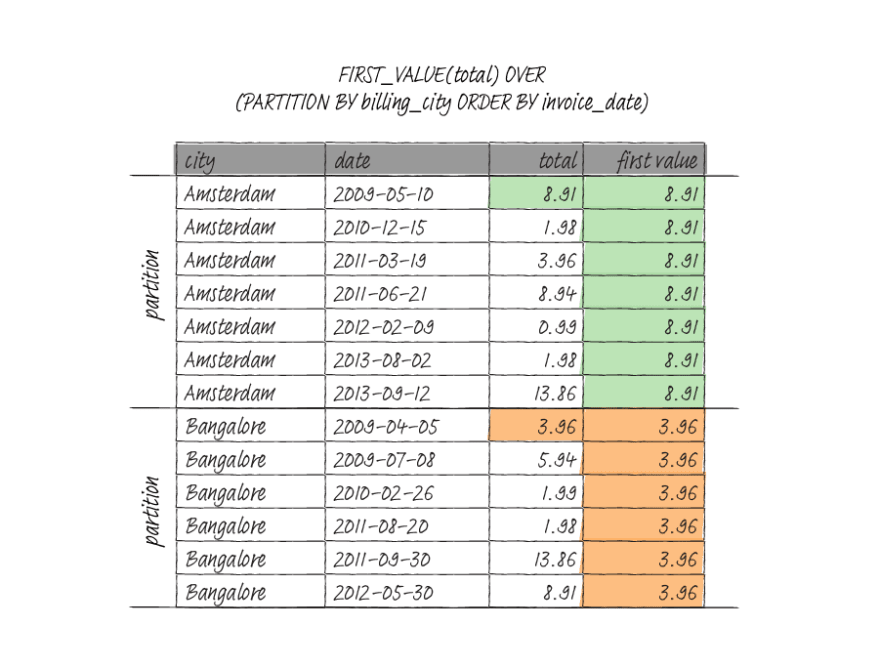
FIRST_VALUE() returns the value for the first row within a window frame.
LAST_VALUE() returns the value for the first row within a window frame. For the last value, you usually want to use RANGE BETWEEN UNBOUNDED PRECEDING AND UNBOUNDED FOLLOWING; otherwise, you will get the current row's value. This behavior is because the default window frame with an ORDER BY clause is between RANGE UNBOUNDED and CURRENT ROW.

The following query partition the data into billing city and fetch the first and last values of the window frame.
SELECT billing_city AS city,
       invoice_date::DATE as date,
       total,
       FIRST_VALUE(total) OVER(
           PARTITION BY billing_city
           ORDER BY invoice_date
       ) as first,
       LAST_VALUE(total) OVER(
           PARTITION BY billing_city
           ORDER BY invoice_date
           RANGE BETWEEN UNBOUNDED PRECEDING
              AND UNBOUNDED FOLLOWING
       ) as last
FROM invoice;
  city        |    date    | total | first | last
-------------------+------------+-------+-------+-------
 Amsterdam    | 2009-05-10 |  8.91 |  8.91 | 13.86
 Amsterdam    | 2010-12-15 |  1.98 |  8.91 | 13.86
 Amsterdam    | 2011-03-19 |  3.96 |  8.91 | 13.86
 Amsterdam    | 2011-06-21 |  8.94 |  8.91 | 13.86
 Amsterdam    | 2012-02-09 |  0.99 |  8.91 | 13.86
 Amsterdam    | 2013-08-02 |  1.98 |  8.91 | 13.86
 Amsterdam    | 2013-09-12 | 13.86 |  8.91 | 13.86
 Bangalore    | 2009-04-05 |  3.96 |  3.96 |  8.91
 Bangalore    | 2009-07-08 |  5.94 |  3.96 |  8.91
 Bangalore    | 2010-02-26 |  1.99 |  3.96 |  8.91
 Bangalore    | 2011-08-20 |  1.98 |  3.96 |  8.91
 Bangalore    | 2011-09-30 | 13.86 |  3.96 |  8.91
 Bangalore    | 2012-05-30 |  8.91 |  3.96 |  8.91
<------------------- TRUNCATED ------------------->
ntile
NTILE(n) divides the partition as equally as possible into n groups and assigns an integer ranging from 1 to n.
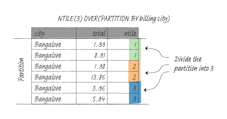
NTILE requires an ORDER BY clause but does not accept window frame definition.
In the following query, I partition the data by billing city and divide each partition into three groups.
SELECT billing_city AS city,
       total,
       NTILE(3) OVER(PARTITION BY billing_city)
FROM invoice;
        city         | total | ntile
--------------------------+-------+-------
 Amsterdam           |  1.98 |     1
 Amsterdam           | 13.86 |     1
 Amsterdam           |  0.99 |     1
 Amsterdam           |  8.91 |     2
 Amsterdam           |  8.94 |     2
 Amsterdam           |  3.96 |     3
 Amsterdam           |  1.98 |     3
 Bangalore           |  1.99 |     1
 Bangalore           |  8.91 |     1
 Bangalore           |  1.98 |     2
 Bangalore           | 13.86 |     2
 Bangalore           |  3.96 |     3
 Bangalore           |  5.94 |     3
<------------- TRUNCATED ----------->
nth value
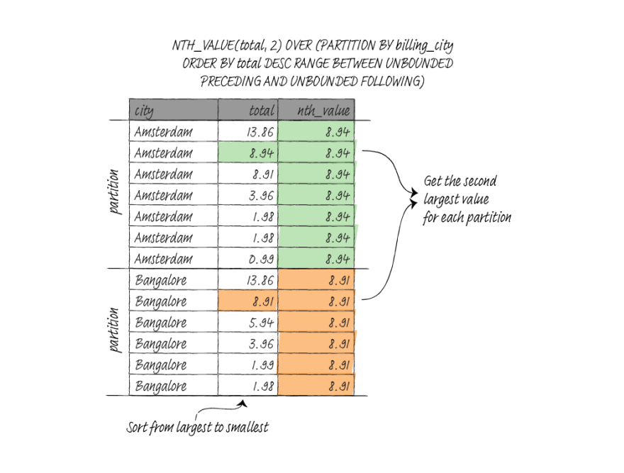
NTH_VALUE(args, n) return values at the nth row of the window frame or NULL if the row does not exist. The counting starts from 1.
ORDER BY is not required, but you need to pay attention to the frame similar to the LAST_VALUE function. If you use the ORDER BY clause, you probably need to specify RANGE BETWEEN UNBOUNDED PRECEDING AND UNBOUNDED FOLLOWING to get the correct value.
In the following query, I partition the data per billing city and sort the total descendingly to get the second largest total for each partition.
SELECT billing_city AS city,
       total,
       NTH_VALUE(total, 2) OVER(
            PARTITION BY billing_city
            ORDER BY total DESC
            RANGE BETWEEN UNBOUNDED PRECEDING AND UNBOUNDED FOLLOWING
        )
FROM invoice;
        city         | total | nth_value
--------------------------+-------+-----------
 Amsterdam           | 13.86 |      8.94
 Amsterdam           |  8.94 |      8.94
 Amsterdam           |  8.91 |      8.94
 Amsterdam           |  3.96 |      8.94
 Amsterdam           |  1.98 |      8.94
 Amsterdam           |  1.98 |      8.94
 Amsterdam           |  0.99 |      8.94
 Bangalore           | 13.86 |      8.91
 Bangalore           |  8.91 |      8.91
 Bangalore           |  5.94 |      8.91
 Bangalore           |  3.96 |      8.91
 Bangalore           |  1.99 |      8.91
 Bangalore           |  1.98 |      8.91
<--------------- TRUNCATED ------------->
Windows function parameter requirement summary
The following table summarizes which window functions require an ORDER BY clause and which functions accept window frame definitions like ROWS, RANGE, and GROUPS.
| Functions | Requires ORDER BY | Accept Window Frame |
|---|---|---|
| avg() | No | Yes |
| count() | No | Yes |
| max() | No | Yes |
| min() | No | Yes |
| sum() | No | Yes |
| row_number() | No | No |
| rank() | Yes | No |
| dense_rank() | Yes | No |
| percent_rank() | Yes | No |
| cume_dist() | Yes | No |
| lead() | Yes | No |
| lag() | Yes | No |
| first_value() | No | Yes |
| last_value() | No | Yes |
| ntile() | Yes | No |
| nth_value() | No | Yes |
Wrap up
In this article, I gave an overview of a handful of windows functions. The window functions I have gone through are split into four categories: aggregate, ranking, distribution, and analytics. In the following article, I will show you several real-world use cases for window functions.


Top comments (0)