One of the machine learning problems is the classification problems.
" Classification is the problem of categorizing observations(inputs) in a different set of classes(category) based on the previously available training-data".
The simplest classification model is the logistic regression model, and today we will attempt to predict if a person will survive on titanic or not. Here, we are going to use the titanic dataset - source.
Variables in Data
Survived - "survived -> 1", "not survived ->0"
Pclass- intuition here is "first class-> 1", "business class->2",
"economy class->3"
Name- it's the passanger's name
Sex- "male->1", "female->0"
Age- passenger's age
Siblings/Spouses Aboard- numbers of siblings/spouses of passenger on the titanic
Parents/Children Aboard- numbers of parents/children of passender on the titanic
Fare- ticket price
Here, the survived variable is what we want to predict, and the rest of the others are the features that we will use for model training.
Firstly, add some python modules to do data preprocessing, data visualization, feature selection and model training and prediction etc.
import pandas as pd
import numpy as np
import matplotlib.pyplot as plt

from sklearn.preprocessing import LabelEncoder
from sklearn.linear_model import LogisticRegression
from sklearn.model_selection import train_test_split
from sklearn.utils import resample

import seaborn as sns
Now, it's time to read data.
raw_data = pd.read_csv('data/titanic.csv', header=0)
raw_data.head()
'DataFrame.head()' is used to get a simple overview of the tabular dataframe.
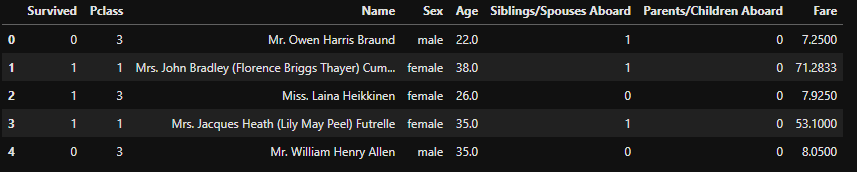
If you observe closely, 'Name' feature is redundant and It's better to remove such idle feature from the dataset also the 'Fare' can be rounded up.
raw_data = raw_data.drop(columns = 'Name')
raw_data['Fare'] = raw_data['Fare'].round(0)
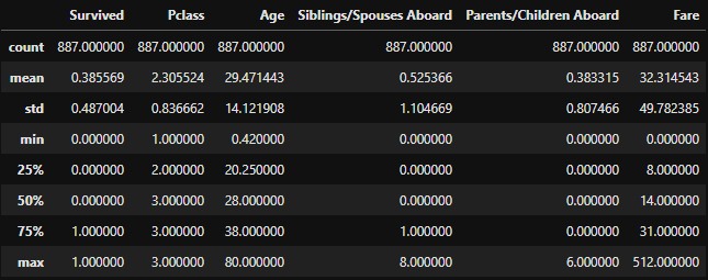
raw_data.describe()
Moving forward, we'll check whether the data is balanced or not because of imbalance the prediction could be biased towards the bigger quantity.
sns.countplot(x='Survived',data=raw_data)
plt.title('Not Survived vs Survived')
plt.show()
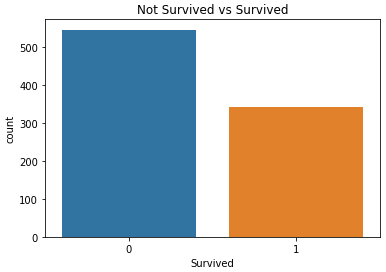
It's imbalanced and we will balance it using SMOTE (Synthetic Minority Oversampling Technique). Before that, we have to handle the categorical data.
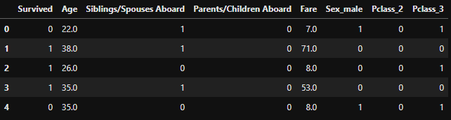
Dummy Variables
In real life datasets, more often we dealt with the categorical and the numerical type of features at the same time. creating dummy variables on categorical data can help us reduce the complexity of the learning process. (otherwise we will have to create different equations for different labels)
In our dataset, 'Sex', 'Pclass' are the two categorical features on which we will create dummy variables(features) and also going to ignore any one of the columns as to avoid collinearity.
Read More on dummy variables
final_data = pd.get_dummies(raw_data, columns =['Sex','Pclass'], drop_first=True)
final_data.head()
Feature selection is one of the important tasks to do while training your model. Here for this dataset, we will not do any feature selection as it's having
887 examples and 7 features only.
Go to my github to see the heatmap on this dataset or RFE can be a fruitful option for the feature selection.
SMOTE
Before the data balancing, we need to split the dataset into a training set (70%) and a testing set (30%), and we'll be applying smote on the training set only. The 'imblearn' module provides a built-in smote function for data balancing.
Read more on SMOTE.
X = final_data.loc[:,final_data.columns != 'Survived']
y = final_data.loc[:,final_data.columns == 'Survived']

from imblearn.over_sampling import SMOTE

X_train, X_test, y_train, y_test = train_test_split(X, y, test_size=0.3, random_state=0)

smt = SMOTE(random_state=0)
data_X,data_y=smt.fit_sample(X_train, y_train)

sns.countplot(x='Survived',data=data_y)
plt.title('Not Survived vs Survived')
plt.show()

Training
For the training, we will be using 'LogisticRegression' method provided by sklearn module and it also helps in testing different parameters of the model as well.
logreg = LogisticRegression(max_iter=500)
logreg.fit(data_X, data_y.values.ravel())

y_pred = logreg.predict(X_test)
print('Accuracy of logistic regression classifier on test set: {:.2f}'.format(logreg.score(X_test, y_test)))
Current model has accuracy of 78%.
Testing
#confusion matrix
from sklearn.metrics import confusion_matrix
confusion_matrix = confusion_matrix(y_test, y_pred)
print(confusion_matrix)

#different perfomance matric
from sklearn.metrics import classification_report
print(classification_report(y_test, y_pred))

#ROC
from sklearn.metrics import roc_auc_score
from sklearn.metrics import roc_curve

logit_roc_auc = roc_auc_score(y_test, logreg.predict(X_test))
fpr, tpr, thresholds = roc_curve(y_test, logreg.predict_proba(X_test)[:,1])
plt.figure()
plt.plot(fpr, tpr, label='Logistic Regression (area = %0.2f)' % logit_roc_auc)
plt.plot([0, 1], [0, 1],'r-')
plt.xlim([0.0, 1.0])
plt.ylim([0.0, 1.0])
plt.xlabel('False Positive Rate')
plt.ylabel('True Positive Rate')
plt.title('ROC')
plt.legend(loc="lower right")
plt.show()
If you don't know what is ROC curve and things like threshold, FPR, TPR. You must
read below given writing

Do comment, if you want to discuss any of the above.


Top comments (0)