
Geometry for Game Programming and Graphics
For the next few lectures, we will discuss some of the basic elements of geometry. While software systems like Unity can conceal many of the issuesinvolving the low-level implementation of geometric primitives, it is important to understand how these primitives can be manipulated in order to achieve the visual results we desire. Computer graphics deals largely with the geometry of lines and linear objects in 3-space, because light travels in straight lines. For example, here are some typical geometric problems that arise in designing programs for computer graphics.
Transformations
You are asked to render a twirling boomerang flying through the air. How would you represent the boomerang’s rotation and translation over time in 3-dimensional space? How would you compute its exact position at a particular time?
Geometric Intersections
Given the same boomerang, how would you determine whether it has hit another object?
Orientation
You have been asked to design the AI for a non-player agent in a flight combat simulator. You detect the presence of a enemy aircraft in a certain direction. How should you rotate your aircraft to either attack (or escape from) this threat?
Change of coordinates
We know the position of an object on a table with respect to a coordinate system associated with the table. We know the position of the table with respect to a coordinate system associated with the room. What is the position of the object with respect to the coordinate system associated with the room?
Reflection and refraction
We would like to simulate the way that light reflects off of shiny objects and refracts through transparent objects.
Such basic geometric problems are fundamental to computer graphics, and over the next few lectures, our goal will be to present the tools needed to answer these sorts of questions. (By the way, a good source of information on how to solve these problems is the series of books entitled “Graphics Gems”. Each book is a collection of many simple graphics problems and provides algorithms for solving them.) There are various formal geometric systems that arise naturally in computer graphics applications.
The principal ones are:
Affine Geometry
The geometry of simple “flat things”: points, lines, planes, line segments, triangles, etc. There is no defined notion of distance, angles, or orientations, however.
Euclidean Geometry
The geometric system that is most familiar to us. It enhances affine geometry by adding notions such as distances, angles, and orientations (such as clockwise and counterclockwise).
Projective Geometry
In Euclidean geometry, there is no notion of infinity (in the same way that in standard arithmetic, you cannot divide by zero). But in graphics, we often need to deal with infinity. (For example, two parallel lines in 3-dimensional space can meet at a common vanishing point in a perspective rendering. Think of the point in the distance where two perfectly straight train tracks appear to meet. Computing this vanishing point involves points at infinity.) Projective geometry permits this.
Affine Geometry
The basic elements of affine geometry are:
- scalars, which we can just think of as being real numbers
- points, which define locations in space
- free vectors (or simply vectors), which are used to specify direction and magnitude, but have no fixed position.
The term “free” means that vectors do not necessarily emanate from some position (like the origin), but float freely about in space. There is a special vector called the zero vector, 0⃗, that has no magnitude, such that v⃗+0⃗=0⃗+v⃗=v⃗.
Note that we did not define a zero point or “origin” for affine space. This is an intentional omission. No point special compared to any other point. (We will eventually have to break down and define an origin in order to have a coordinate system for our points, but this is a purely representational necessity, not an intrinsic feature of affine space.)
You might ask, why make a distinction between points and vectors? (Note that Unity does not distinguish between them. The data type Vector3 is used to represent both.) Although both can be represented in the same way as a list of coordinates, they represent very different concepts. For example, points would be appropriate for representing a vertex of a mesh, the center of mass of an object, the point of contact between two colliding objects. In contrast, a vector would be appropriate for representing the velocity of a moving object, the vector normal to a surface, the axis about which a rotating object is spinning. (As computer scientists the idea of different abstract objects sharing a common representation should be familiar. For example, stacks and queues are two different abstract data types, but they can both be represented as a 1-dimensional array.)
Because points and vectors are conceptually different, it is not surprising that the operations that can be applied to them are different. For example, it makes perfect sense to multiply a vector and a scalar. Geometrically, this corresponds to stretching the vector by this amount. It also makes sense to add two vectors together. This involves the usual head-to-tail rule, which you learn in linear algebra. It is not so clear, however, what it means to multiply a point by a scalar. (For example, the top of the Washington monument is a point. What would it mean to multiply this point by 2?) On the other hand, it does make sense to add a vector to a point. For example, if a vector points straight up and is three meters long, then adding this to the top of the Washington monument would naturally give you a point that is three meters above the top of the monument.
We will use the following notational conventions. Points will usually be denoted by lower-case Roman letters such as p, q, and r. Vectors will usually be denoted with lower-case Roman letters, such as u, v, and w, and often to emphasize this we will add an arrow (e.g., u⃗, v⃗, w⃗). Scalars will be represented as lower case Greek letters (e.g., α, β, γ). In our programs, scalars will be translated to Roman (e.g., a, b, c). (We will sometimes violate these conventions, however. For example, we may use c to denote the center point of a circle or r to denote the scalar radius of a circle.)
Affine Operations
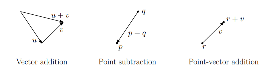
The table below lists the valid combinations of scalars, points, and vectors. The formal definitions are pretty much what you would expect. Vector operations are applied in the same way that you learned in linear algebra. For example, vectors are added in the usual “tail-to-head” manner the following. The difference p−q of two points results in a free vector directed from q to p.
Point-vector addition r + v⃗ is defined to be the translation of r by displacement v⃗. Note that some operations (e.g. scalar-point multiplication, and addition of points) are explicitly not defined.
vector ← scalar · vector, vector ← vector/scalar //scalar-vector multiplication
vector ← vector + vector, vector ← vector − vector //vector-vector addition
vector ← point − point //point-point difference
point ← point + vector, point ← point − vector //point-vector addition
```
### Affine Combinations
Although the algebra of affine geometry has been careful to disallow point addition and scalar multiplication of points, there is a particular combination of two points that we will consider legal. The operation is called an affine combination.
Let’s say that we have two points _p_ and _q_ and want to compute their midpoint _r_, or more generally a point _r_ that subdivides the line segment p⃗q into the proportions _α_ and _**1 − α**_, for some _**α ∈ [0, 1]**_.
(The case _**α = 1/2**_ is the case of the midpoint). This could be done by taking the vector _q − p_, scaling it by _α_, and then adding the result to _p_. That is,
_**r = p + α(q − p)**_
Another way to think of this point _r_ is as a _weighted average_ of the endpoints _p_ and _q_. Thinking of _r_ in these terms, we might be tempted to rewrite the above formula in the following (technically illegal) manner:
_**r = (1 − α)p + αq**_
Observe that as α ranges from _0_ to _1_, the point r ranges along the line segment from _p_ to _q_. In fact, we may allow to become negative in which case _r_ lies to the left of _p_, and if _**α > 1**_, then _r_ lies to the right of _q_. The special case when _**0 ≤ α ≤ 1**_, this is called a _convex combination_.
In general, we define the following two operations for points in affine space.
#### Affine combination
Given a sequence of points _**p<sub>1</sub>, p<sub>2</sub>, . . . , p<sub>n</sub>,**_ an affine combination is any sum of
the form;
_**α<sub>1</sub>p<sub>1</sub> + α<sub>2</sub>p<sub>2</sub> + . . . + α<sub>n</sub>p<sub>n</sub>**_
where _**α1, α2, . . ., αn**_ , are scalars satisfying _**Σ<sub>i</sub>α<sub>i</sub> = 1**_ .

#### Convex combination
Is an affine combination, where in addition we have _**α<sub>i</sub> ≥ 0**_ for _**1 ≤ i ≤ n**_.
Affine and convex combinations have a number of nice uses in graphics. For example, any three noncollinear points determine a plane. There is a _1–1_ correspondence between the points on this plane and the affine combinations of these three points. Similarly, there is a _1–1_ correspondence between the points in the triangle determined by the these points and the _convex combinations_ of the points. In particular, the point **(1/3)p + (1/3)q + (1/3)r** is the centroid of the triangle.
We will sometimes be sloppy, and write expressions like **(p + q)/2**, which really means **(1/2)p + (1/2)q**. We will allow this sort of abuse of notation provided that it is clear that there is a legal affine combination that underlies this operation.
To see whether you understand the notation, consider the following questions. Given three points in the 3-space, what is the union of all their affine combinations? (Ans: the plane containing the 3 points.) What is the union of all their convex combinations? (Ans: The triangle defined by the three points and its interior.)
#### Euclidean Geometry
In affine geometry we have provided no way to talk about angles or distances. Euclidean geometry is an extension of affine geometry which includes one additional operation, called _the inner product_.
The inner product is an operator that maps two vectors to a scalar. The product of **u⃗** and **v⃗** is denoted commonly denoted (**u⃗**, **v⃗**). There are many ways of defining the inner product, but any legal definition should satisfy the following requirements
**Positiveness:** (**u⃗**, **u⃗**) **≥ 0** and (**u⃗**, **u⃗**) **=** **0** if and only if **u⃗ = 0⃗**.
**Symmetry:** (**u⃗**, **v⃗**) = (**v⃗**, **u⃗**).
**Bilinearity:** (**u⃗**, **v⃗** **+ w⃗**) **=** (**u⃗**, **v⃗**) **+** (**u⃗**, **w⃗**), and (**u⃗**, **α⃗v**) = **α**(**u⃗**, **v⃗**). (Notice that the symmetric forms follow by symmetry.)
> For more information, you can take a look at the explanations about linear algebra. Here I leave some useful resources for you.
> - [MATH 233 - Linear Algebra I Lecture Notes | Cesar O. Aguilar](https://www.geneseo.edu/~aguilar/public/assets/courses/233/main_notes.pdf)
> - [Linear Algebra in Twenty Five Lectures | Tom Denton and Andrew Waldron](https://www.math.ucdavis.edu/~linear/linear.pdf)
> - [The Geometry of Linear Equations | MIT Open Course Ware](https://ocw.mit.edu/courses/mathematics/18-06sc-linear-algebra-fall-2011/ax-b-and-the-four-subspaces/the-geometry-of-linear-equations/)
> - [Notes on Linear Algebra | Peter J. Cameron](http://www.maths.qmul.ac.uk/~pjc/notes/linalg.pdf)
> - [MA106 Linear Algebra lecture notes | Martin Bright and Daan Krammer](https://homepages.warwick.ac.uk/~masbal/LinAlg1011/lectures.pdf)
We will focus on a the most familiar inner product, called the dot product. To define this, we will need to get our hands dirty with coordinates. Suppose that the d-dimensional vector **u⃗** is represented by the coordinate vector (**u<sub>0</sub>, u<sub>2</sub>, . . . , u<sub>d-1</sub>**). Then define;

Note that inner (and hence dot) product is defined only for vectors, not for points. Using the dot product we may define a number of concepts, which are not defined in regular affine
geometry. Note that these concepts generalize to all dimensions.
**Length:** of a vector ~v is defined to be **||v⃗|| =√v⃗ · v⃗**.
**Normalization:** : Given any nonzero vector **v⃗**, define the normalization to be a vector of unit length that points in the same direction as **v⃗**, that is, **v⃗**/||**v⃗**||. We will denote this by **ṽ**.
**Distance between points:** _dist(p, q) = ||p − q||_
**Angle:** between two nonzero vectors **u⃗** and **v⃗** (ranging from _**0**_ to _**π**_) is

This is easy to derive from the law of cosines. Note that this does not provide us with a signed angle. We cannot tell whether **u⃗** is clockwise our counterclockwise relative to **v⃗**. We will discuss signed angles when we consider the cross-product.
**Orthogonality:** **u⃗** and **v⃗** are orthogonal (or perpendicular) if **u⃗ · v⃗ = 0**
**Orthogonal projection:** Given a vector **u⃗** and a nonzero vector **v⃗**, it is often convenient to decompose **u⃗** into the sum of two vectors **u⃗ =u⃗<sub>1</sub> + u⃗<sub>2</sub>**, such that **u⃗<sub>1</sub>** is parallel to **v⃗** and **u⃗<sub>2</sub>** is orthogonal to **v⃗**.

(As an exercise, verify that **u⃗<sub>2</sub>** is orthogonal to **v⃗**.) Note that we can ignore the denominator if we know that **v⃗** is already normalized to unit length. The vector **u⃗<sub>1</sub>** is called the orthogonal projection of **u⃗** onto **v⃗**.


Top comments (1)
Understanding geometry is essential for game programming and graphics because it forms the foundation for simulating realistic movements, interactions, and visual effects in 3D space—whether it's calculating transformations for a spinning object or determining line intersections for collisions. Concepts like affine and Euclidean geometry allow developers to precisely position and orient models, while projective geometry helps in rendering scenes with accurate depth and perspective. A great way to see these geometric principles in action is through games like Geometry Dash, which, despite its simple appearance, relies heavily on timing, spatial awareness, and vector-based movement to create challenging and visually engaging gameplay.
Some comments may only be visible to logged-in visitors. Sign in to view all comments.