Introduction

Natural Language Processing requires sequential data processing and data at any particular time may/may not be related to data sent at earlier time interval. This makes NLP bit complex compare to computer vision problem as network needs to remember relevant data from earlier Input. Question here is that, How we define what is relevant for network to memorize and does this memory requires to evolve as we get more input?
We have RNN, LSTM, GRU and then Attention Model to support NLP in better way.

Limitation of RNN and why so?

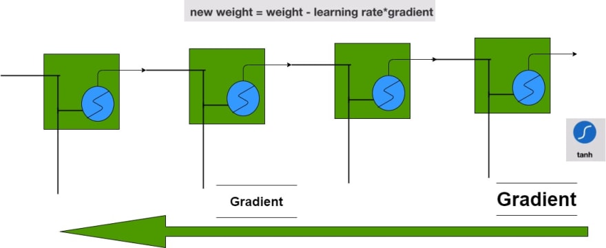
RNN has been the starting of NLP and it takes the basic human capability of sequential data processing where output at timestep t is being fed into timestep t+1 along with input at timestep t+1 for prediction at timestep t+1. This causes issue of vanishing gradient for RNN.

LSTM and Context Memory

LSTM uses memory to store the relevent contextual information and then add/modify/delete contextual information based on new Input. This helps network to predict well for new input when context from very old input will be required to be referred.

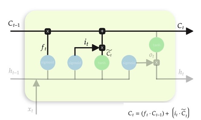
The key to LSTMs is the cell state or memory and following are the other key components of the network. The LSTM cell is mainly composed of 3 gates which are forget, input and output gates as well as the cell state.

Key Benefits are:

• Can remember longer sequence due to presence of Context
• Network takes following inputs
  • Input at the Current time step
  • Output from previous LSTM Unit
  • Cell state/Memory of previous LSTN Unit
• Forget gate is responsible for deleting irrelevant information from memory
• Input gate is responsible to decide relevant information to be added from Input
• Output gates provides hidden state to next LSTM Unit

Cell State

Maintains a vector C(t) that is the same dimensionality as the hidden state, h(t). Information can be added or deleted from this state vector via the forget and input gates.

So lets say that, we want to remember person & number of a subject noun so that it can be checked to agree with the person & number of verb when it is eventually encountered.

• Forget gate will remove existing information of a prior subject when a new one is encountered.

• Input gate "adds" in the information for the new subject.

Cell state is updated by using component-wise vector multiply to "forget" and vector addition to "input" new information. The cell state is known as the memory of the LSTM, it is updated by the forget gate and the input gate.

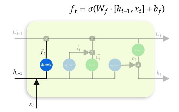
Forget Gate

a neural network with sigmoid)

Forget the additional information which might have entered in the immediate last step, and maintain the long term information required. This is why it is called Forget Gate. The reason of sigmoid gate here is that the value of sigmoid vary between 0 and 1. So any information which needs to be retained will get value from sigmoid gate closer to 1 and information which needs to be forget gets value of 0 from sigmoid.

Multiplicatively combined with cell state, "forgetting" information where the gate outputs something close to 0.

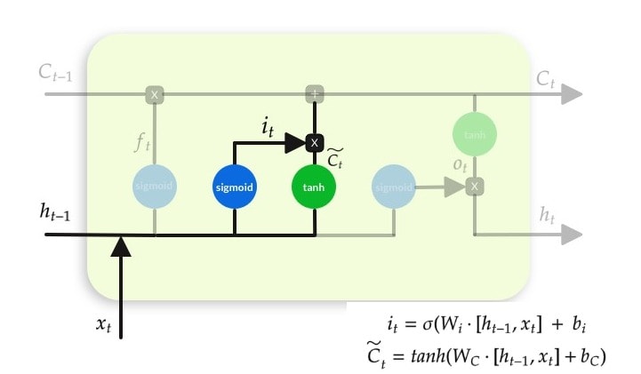
Input Gate

Candidate layer “C`"(a NN with Tanh) and Input Gate “I” ( a NN with sigmoid )

We want to add based on the new-input. For this, we will use 1 DNN to predict all possible values, and other re-scores or filter-outs the values, like a manager, would.

Tanh Gate:

• Tanh can be used as an alternative nonlinear function to the sigmoid logistic (0-1) output function.
• Used to produce thresholded output between –1 and 1.

Now we Update the Memory/Context/Cell-State by multiplicative operation of output from Tanh and sigmoid gate.

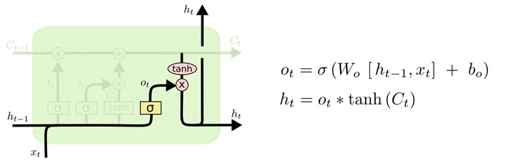
Output Gate

Hidden state is updated based on a "filtered" version of the cell state, scaled to –1 to 1 using tanh. Output gate computes a sigmoid function of the input and current hidden state to determine which elements of the cell state to "output".

How it is in Pytorch

Lets now understand how it is being done in pytorch torch.nn.LSTM function. In order to be initialized, LSTM class needs two important parameters during initialization.

• input_size – The number of expected features in the input x

• hidden_size – The number of features in the hidden state h

• num_layers – Number of recurrent layers. E.g., setting num_layers=2 would mean stacking two LSTMs together to form a stacked LSTM, with the second LSTM taking in outputs of the first LSTM and computing the final results. Default: 1

The LSTM cell needs following input during processing.

• input of shape (batch, input_size): tensor containing input features

• h_0 of shape (batch, hidden_size): tensor containing the initial hidden state for each element in the batch.

• c_0 of shape (batch, hidden_size): tensor containing the initial cell state for each element in the batch.

If (h_0, c_0) is not provided, both h_0 and c_0 default to zero.

The LSTM returns the output and a tuple of the final hidden state and the final cell state, whereas the standard RNN only returned the output and final hidden state. Implementing bidirectionality and adding additional layers are done by passing values for the num_layers and bidirectional arguments for the RNN/LSTM.

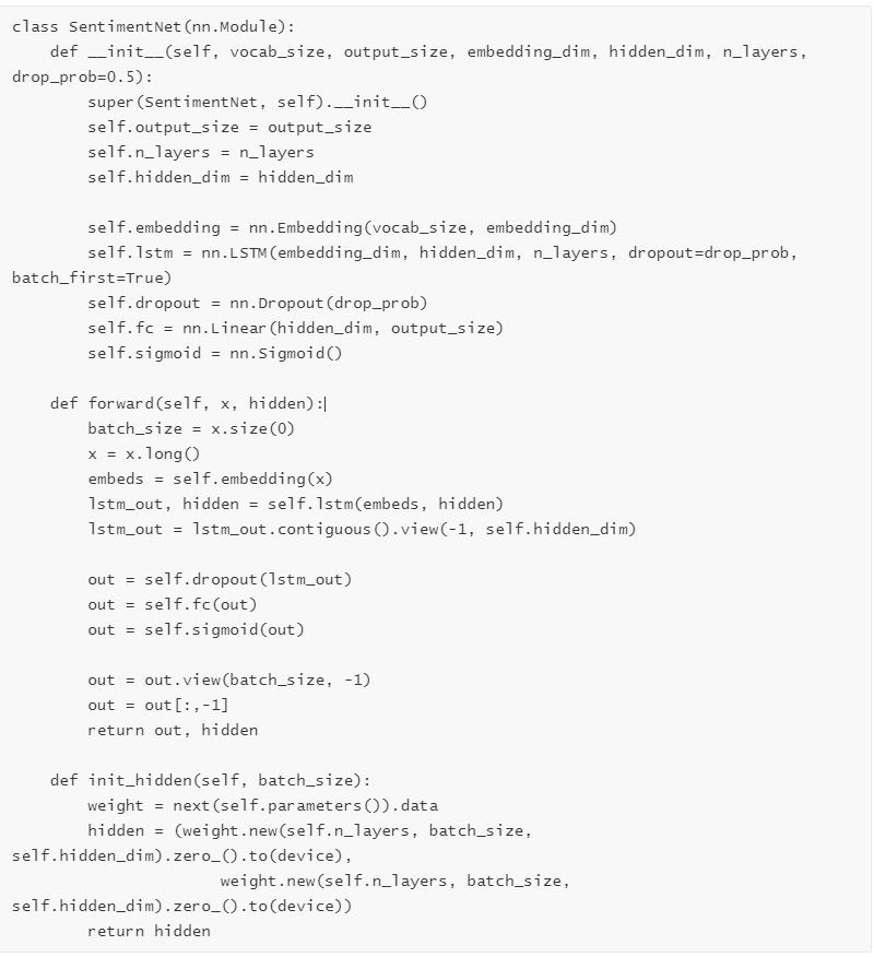
A simple LSTM class definition will look like as follows. Salient points of this network architecture are:

• Base class always needs to be inherited from nn.Module to ensure we get all the pytorch NN Module functions
• LSTM layer has bi-directional set to False and it is a multi-layer LSTM with drop out in-between layers’
• A Fully connected network layer gets input from LSTM layer output after passing through dropout layer
• LSTM hidden layer is being initialized.

So in a nutshell LSTM helps us with

• Context creation
• Deletion from Context
• Update into Context

LSTM Bidirectional

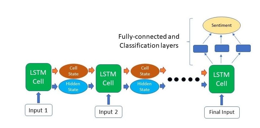
Bidirectional is a boolean input into torch.nn.LSTM which forced LSTM network to train with original input and reversed input. Output of two networks are then concatenated at each time step. This helps to achieve better accuracy as network context becomes richer. But it can’t be used in situations where a sequence model is used for inference (Ex: Machine translation).

Sample Use Case: Sentiment analysis task where a model is trying to classify sentences as positive or negative. Bidirectional models can effectively “look forward” in the sentence to see if “future” tokens may influence the current decision.

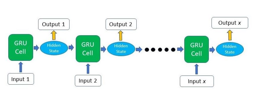
Why GRU?

It is variant of LSTM and no of parameter is less than LSTM. So it trains faster. GRU allows it to adaptively capture dependencies from large sequences of data without discarding information from earlier parts of the sequence. This is achieved through its gating units, similar to the ones in LSTMs.

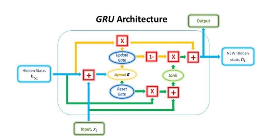
• Combines forget and input gates into Update gate
  • This gate is computed using the previous hidden state and current input data.
• Eliminates cell state vector by Reset gate
  • Update memory using previous hidden state and new input.
  • It then sum them before passing the sum through a sigmoid function
  • The sigmoid function will help filter less important values (by values close to 0) and more important values (by value close to 1).

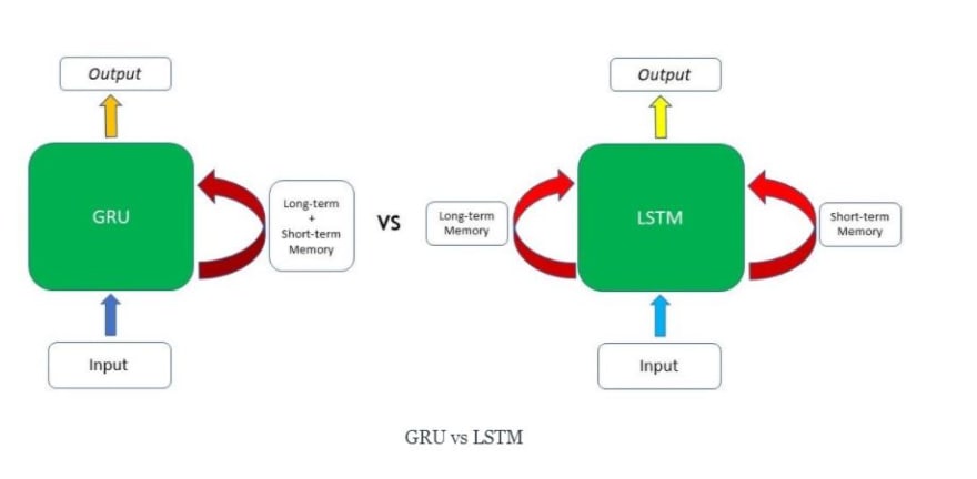
LSTMs have two different states passed between the cells — the cell state and hidden state, which carry the long and short-term memory, respectively — GRUs only have one hidden state transferred between time steps. This hidden state is able to hold both the long-term and short-term dependencies at the same time due to the gating mechanisms and computations that the hidden state and input data go through. This helps to train GRU faster as number of parameter is less.

GRU maintain long-term and short-term memory into same vector while LSTM maintain separate vector.

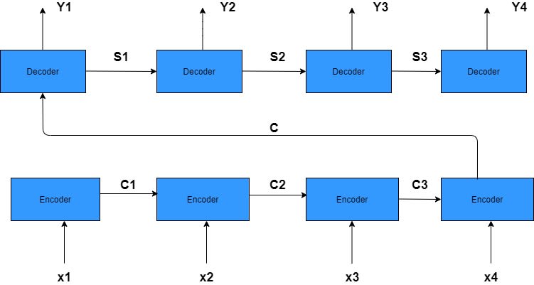
Encoder Decoder - Sequence to Sequence Architecture

• The RNN encoder has an input sequence x1, x2, x3, x4.

• Encoder and Decoder are single layered RNN.

• Encoder states by c1, c2, c3. The encoder outputs a single output vector c which is passed as input to the decoder.

• Decoder states are indicated by s1, s2, s3

• Decoder network’s output by y1, y2, y3, y4.

A potential issue with this encoder–decoder approach is that a neural network needs to be able to compress all the necessary information of a source sentence into a fixed-length vector. This may make it difficult for the neural network to cope with long sentences, especially those that are longer than the sentences in the training corpus.

How Attention aspect works better?

The basic idea: each time the model predicts an output word, it only uses parts of an input where the most relevant information is concentrated instead of an entire sentence. In other words, it only pays attention to some input words. Encoder can not be a bidirectional LSTM.

In a nutshell, attention in deep learning can be broadly interpreted as a vector of importance weights: in order to predict or infer one element, such as a pixel in an image or a word in a sentence, we estimate using the attention vector how strongly it is correlated with (or “attends to” as we may have read in many papers) other elements and take the sum of their values weighted by the attention vector as the approximation of the target.

• For many applications, it helps to add “attention” to RNNs.

• Allows network to learn to attend to different parts of the input at different time steps, shifting its attention to focus on different aspects during its processing.

• Used in image captioning to focus on different parts of an image when generating different parts of the output sentence.

Why it works better compare to LSTM/GRU?

• It sends entire sequence of all the LSTM unit output to Attention Layer instead of only sending last LSTM Unit hidden state/output for understanding in LSTM/GRU
• Produces softmax values to indicate attention probability like values
• 

Key Points

• single layer RNN encoder with 4-time steps
• Encoder’s input vectors by x1, x2, x3, x4
• Encoder’s output vectors by h1, h2, h3, h4
• Attention mechanism input composed of the encoder’s output vectors h1, h2, h3, h4 and the states of the decoder s0, s1, s2, s3
• Attention’s output is a sequence of vectors named context vectors denoted by c1, c2, c3, c4

The context vectors enable the decoder to focus on certain parts of the input when predicting its output

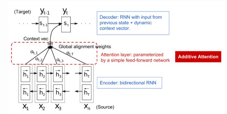
Attention Network Building Block

The attention mechanism developed to help memorize long source sentences in neural machine translation. Rather than building a single context vector out of the encoder’s last hidden state, the secret sauce invented by attention is to create shortcuts between the context vector and the entire source input. The weights of these shortcut connections are customizable for each output element.

The context vectors enable the decoder to focus on certain parts of the input when predicting its output. The attention weights are learned using an additional fully connected shallow network. The attention weights are learned using the attention fully-connected network and a softmax function:

References

Credit goes to Fernando López and Rohan Shravan for their outstanding blogs and lecture notes.