Text in natural scene images usually carries abundant semantic information. However, due to variations of text and complexity of background, detecting text in scene images becomes a critical and challenging task. This algorithm consists of a fully convolutional network with a non-max suppression (NMS) merging state. The paper proposes a scene text detection method that consists of two stages: Fully Convolutional Network and an NMS merging stage. The FCN directly produces text regions, excluding redundant and time-consuming intermediate steps

Every single shot object detector has 3 major stages involved:
- Feature extraction stage.
- Feature fusion stage.
- Prediction network.

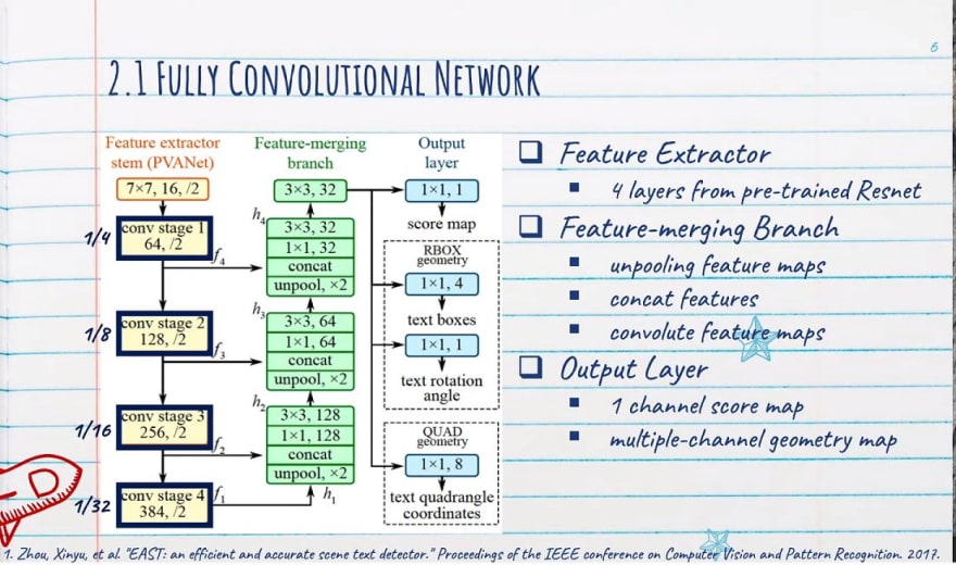
The model is a fully-convolutional neural network adapted for text detection that outputs dense per-pixel pre-dictions of words or text lines. This eliminates intermediate steps such as candidate proposal, text region formation and word partition. The post-processing steps only include thresholding and NMS on predicted geometric shapes. The detector is named as EAST, since it is an Efficient and Accuracy Scene Text detection pipeline.
Authors have experimented with two geometry shapes for text regions, rotated box (RBOX) and quadrangle (QUAD),and designed different loss functions for each geometry. Thresholding is then applied to each predicted region,where the geometries whose scores are over the predefined threshold is considered valid and saved for later non-maximum-suppression. Results after NMS are considered the final output of the pipeline.
Recap of Some basics
Pooling and Unpooling
It is essential to recap Pooling and Unpooling before we jump into network architecture.
What does Pooling do?
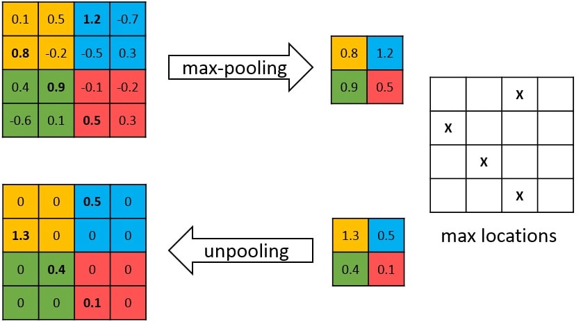
Pooling in convolutional network is designed to filter noisy activations, it helps by retaining only robust activations in upper layers, but the spatial information is lost during pooling.
The convolution network corresponds to feature extractor that transforms the input image to multidimensional feature representation, the deconvolution network is a shape generator that produces object segmentation from feature extracted from the convolution network.
Unpooling layer
During the pooling operation, create a matrix which record the location of the maximum value, unpool operation will insert the pooled value in the original place, with the remaining elements being set to zero. Unpooling captures example-specific structures by tracing the original locations with strong activations back to image space. As a result, it effectively reconstructs the detailed structure.

Architecture
Basic Network
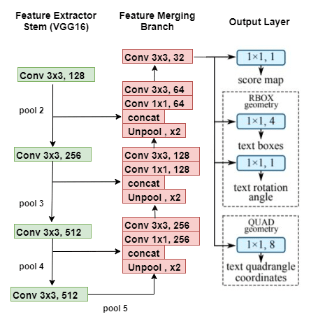
- The network takes in an input image and passed through some set of conv layers(feature extractor stem) to get four levels of feature maps — f1, f2, f3, f4.
The feature maps are then unpooled(x2), concatenated(along channel dimension) and then passed through 1x1 followed by 3x3 convs. The reason for merging features from different spatial resolution is to predict smaller word regions.
The final feature volume will be then used to make score and box predictions — 1x1 filter of depth=1 used to generate score map, another 1x1 filter of depth=5 is used to generate RBOX(rotated boxes) — four box offsets and rotation angle, and another 1x1 filter of depth=8 to generate QUAD(quadrangle with 8 offsets).
Feature Extractor component
This branch of the network is used to extract features from different layers of the network. This stem can be a convolutional network pretrained on the ImageNet dataset. Authors of EAST architecture used PVANet and VGG16 both for the experiment.
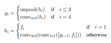
In this blog, we will see EAST architecture with the VGG16 network only. Let’s see the architecture of the VGG16 model. For the stem of architecture, it takes the output from the VGG16 model after pool2, pool3, pool4, and pool5 layers.

It has also been observed that
- No of convolution channel in each layer is being increased by multiple of 2
- Authors have kept number of channels for convolutions in branch small, which adds only a fraction of computation overhead over the stem, making the network computation-efficient
Feature Merging component
In this branch of the EAST network, it merges the feature outputs from a different layer of the VGG16 network. The input image is passed through the VGG16 model and outputs from different four layers of VGG16 are taken. Merging these feature maps will be computationally expensive. That’s why EAST uses a U-net architecture to merge feature maps gradually (see EAST architecture figure). Firstly, outputs after the pool5 layer are upsampled using a deconvolutional layer. Now the size of features after this layer would be equal to outputs from the pool4 layer and both are then merged into one layer. Then Conv 1×1 and Conv 3×3 are applied to fuse the information and produce the output of this merging stage.
For the stem of architecture, it takes the output from the VGG16 model after pool2, pool3, pool4, and pool5 layers.
Four levels of feature maps, denoted as f(i),are extracted from the stem, whose sizes are1/32, 1/16, 1/8 and 1/4 of the input image, respectively.
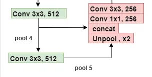
Feature merging architecture is repeating one and it has concatenated two set of feature after previous one have gone through Unpooling. Conv 1x1 has been used here to reduce number of channel and then it has gone through Conv 3x3. The paper states:
- In each merging stage, the feature map from the last stage is first fed to an unpooling layer to double its size
- then concatenated with the current feature map
- Next, a conv1×1 bottleneck cuts down the number of channels and reduces computation
- It then followed by aconv3×3that fuses the information to finally produce the output of this merging stage
Following the last merging stage, a conv3×3 layer produces the final feature map of the merging branch and feed it to the output layer.
It has also been observed that
- No of output channel is being reduced gradually starting from 128 to 32. This is the reason of using 1x1 filter.
Output Layer
The output layer consists of a score map and a geometry map. The score map tells us the probability of text in that region while the geometry map defines the boundary of the text box. This geometry map can be either a rotated box or quadrangle. A rotated box consists of top-left coordinate, width, height and rotation angle for the text box. While quadrangle consists of all four coordinates of a rectangle.
The final output layer contains several conv1×1operations to project 32 channels of feature maps into 1 channel of score maps and a multi-channel geometry map. The geometry output can be either one of RBOX or QUAD.
Thresholding and MMS being used to merge bounding boxes.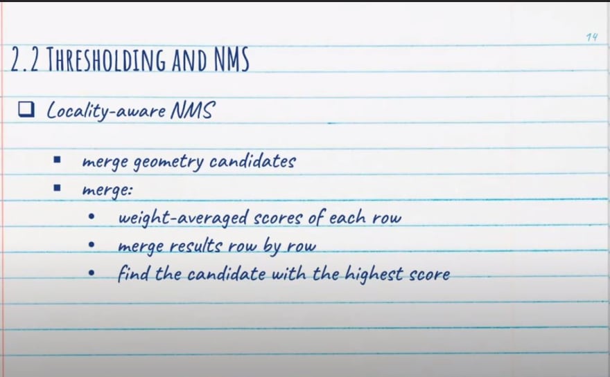
It has also been observed that
- RBOX, the geometry is represented by 4 channels of axis-aligned bounding box (AABB) R and 1 channel rotation angleθ . The formulation of R is where the 4 channels represents 4 distances from the pixel location to the top, right, bottom, left boundaries of the rectangle respectively.

- For the detected shape is QUAD, the output contains the score map and the text shape (eight offsets from the corner vertices), that is, there are 9 outputs together, of which QUAD has 8 values.

Loss function
The loss function of such network will have two component. First component is due to Prediction for object presence and 2nd one is due to co-ordinates of the bounding boxes. 
For RBOX, the main tasks include text confidence regression (get score map), border offset regression (geometry map), and angular offset regression (θ theta θ map). The total loss function of the network is:

Loss for Score Map
Different from the common target detection network to deal with sample imbalance, such as equalization sampling, OHEM and so on. EAST algorithm is adopted Class balanced cross entropy to solve the problem of category imbalance.
where β weighting is used, the weight is determined by the ratio of positive and negative cases, and the smaller the ratio, the larger the weight. But in the actual combat, generally adopted dice loss because its convergence speed will be faster than the class balance cross entropy.

Loss for Geometries
The paper says “Directly using L1 or L2 loss for regression would guide the loss bias towards larger and longer text regions”. So they found that, in order to generate accurate text geometry prediction for both large and small text regions, the regression loss should be scale-invariant. Therefore authors have adopted the IoU loss in the AABB part of RBOX regression, and a scale-normalized smoothed-L1 loss for QUAD regression.

RBOX offset angle loss
RBOX also has an angle, here uses the cosine loss:

The hats in the above formula all indicate predictions, and "*" means GT. and so:
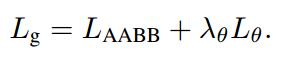
Whereλθ is set to10 in authors experiments.
Locality-Aware NMS
Predicted geometries after fully convolutional network are passed through a threshold value. After this thresholding, remaining geometries are suppressed using a locality aware NMS. A Naive NMS runs in O(n2) where n is the number of candidate geometries, which is unacceptable as we are facing tens of thousands of geometries from dense predictions. But to run this in O(n), authors adopted a method which uses suppression row by row. This row by row suppression also takes into account iteratively merging of the last merged one. This makes this algorithm fast in most of the cases but the worst time complexity is still O(n2).
Based on Hypothesis: Candidate boxes based on adjacent pixels are highly correlated. Therefore, these candidate boxes can be merged step by step, and then the conventional NMS.
Training
The network is trained end-to-end using ADAM optimizer. To speed up learning, they have uniformly sampled 512x512 crops from images to form a minibatch of size 24.
Learning rate of ADAM starts from 1e-3, decays to one-tenth every 27300 minibatches, and stops at 1e-5.
Limitations
The maximal size of text instances the detector can handle is proportional to the receptive field of the network. This limits the capability of the network to predict even longer text regions like text lines running across the images. Also, the algorithm might miss or give imprecise pre-dictions for vertical text instances as they take only a small portion of text regions in the ICDAR 2015 training set.


Top comments (0)