A Nested Loop join is a loop reading rows from the outer table and, nested within this loop, another loop on the inner table to read rows that matches the join criteria.
From a performance point of view, the number of rows from the outer table multiplies the time to access to the inner table. This is acceptable for few rows. Imagine an OLTP query like "return the 10 past orders for one customer": one outer loop only, from customers, and an index access to the orders.
When the join reads lot of rows, a Hash Join is usually preferred. Imagine a reporting query like "return all orders from last month with their product information". This reads all products, hash it in memory, then reads the last orders partition and use the hash table to add the product information.
There are many cases that are in the middle, where reading all rows to do a Hash Join is too much, but thousand of nested loops is also too expensive. And what is too expensive in a monolithic database is worse is an distributed database: more network transfer for Hash Join, or more network calls for Nested Loops.
The optimization for this situation is still work in progress for YugabyteDB, I'm writing this for version 2.13, and is tracked by [YSQL] Improve the performance of NestedLoop joins with Index Scans using batched execution #4903
Example
In a lab, I create the following two tables that I'll will join on (a1,b1):
drop table if exists a,b;
create table a(a1 int, a2 int, primary key(a1,a2), x int);
create index ax on a(x,a1,a2);

create table b(a1 int, a2 int, b int
 , primary key(a1 asc, a2 asc, b))
split at values ((333,0),(666,0));

insert into a select  a1, a2, mod(a1,10) from generate_series(1,1000) a1, generate_series(1,10) a2;
insert into b select a1, a2, b from a , generate_series(1,10) b;
analyze a, b;
I also load my ybwr.sql to show the number of rocksdb seek() and next() in the tservers:
\! curl -s https://raw.githubusercontent.com/FranckPachot/ybdemo/main/docker/yb-lab/client/ybwr.sql | grep -v '\watch' > ybwr.sql
\i ybwr.sql
Hash Join
Here is my query selecting rows=1000 rows from table a (where x = 0) and joining on ((b.a1 = a.a1) AND (b.a2 = a.a2)) to get the rows=10000 matching rows from b:
yugabyte=# explain (costs off, analyze)
           select * from a natural join b where a.x=0;

                                       QUERY PLAN
----------------------------------------------------------------------------------------
 Hash Join (actual time=12.511..410.649 rows=10000 loops=1)
   Hash Cond: ((b.a1 = a.a1) AND (b.a2 = a.a2))
   ->  Seq Scan on b (actual time=3.900..375.657 rows=100000 loops=1)
   ->  Hash (actual time=8.289..8.289 rows=1000 loops=1)
         Buckets: 1024  Batches: 1  Memory Usage: 51kB
         ->  Index Only Scan using ax on a (actual time=7.745..8.148 rows=1000 loops=1)
               Index Cond: (x = 0)
               Heap Fetches: 0
 Planning Time: 10.434 ms
 Execution Time: 411.152 ms

yugabyte=# execute snap_table;

 rocksdb_#_db_seek | rocksdb_#_db_next |         dbname / relname / tserver / tabletid
-------------------+-------------------+--------------------------------------------------------
                 1 |              1000 | yugabyte ax 10.0.0.62 bde34094405741109c209699567e8a6f
                33 |             33331 | yugabyte b 10.0.0.61 c886d0ad76eb472fb222862c231e2e7e
                33 |             33531 | yugabyte b 10.0.0.62 32c443ea5ebd441c890e96a73dac6cf4
                33 |             33231 | yugabyte b 10.0.0.63 271e183b13a44568860143fe1dbce5d8
(4 rows)
I'm interested by the access to table b. The full table scan Seq Scan on b (actual time=3.900..375.657 rows=100000 loops=1) reads all rows, and returns all of them to the SQL processing nodes. We measured a total of 100 seek() and 100000 next() calls in the LSM-tree to get these 100000 values, transferred from the 3 tablet servers to be filtered out by the postgres backend, which will probe the build table by hash, to get the 10000 rows of the result. I am on a lab with all nodes on the same machine, and even with this minimal network latency, the execution time is 410.649 milliseconds, mainly from the 375.657ms of Seq Scan. With a real deployment, the network transfer of those 100000 will add to the response time (and to the cloud service bill).
Nested Loop
If I force a Nested Loop from a to b I have rows=1000 rows returned by the outer loop and calling loops=1000 inner loops:
yugabyte=# explain (costs off, analyze)
           /*+ Leading((a b)) NestLoop(a b) */
           select * from a natural join b where a.x=0;

                                    QUERY PLAN
----------------------------------------------------------------------------------
 Nested Loop (actual time=5.047..505.595 rows=10000 loops=1)
   ->  Index Only Scan using ax on a (actual time=4.261..5.363 rows=1000 loops=1)
         Index Cond: (x = 0)
         Heap Fetches: 0
   ->  Index Scan using b_pkey on b (actual time=0.482..0.487 rows=10 loops=1000)
         Index Cond: ((a1 = a.a1) AND (a2 = a.a2))
 Planning Time: 0.179 ms
 Execution Time: 506.318 ms
(8 rows)

yugabyte=# execute snap_table;

 rocksdb_#_db_seek | rocksdb_#_db_next |         dbname / relname / tserver / tabletid
-------------------+-------------------+--------------------------------------------------------
                 1 |              1000 | yugabyte ax 10.0.0.62 bde34094405741109c209699567e8a6f
               330 |              3300 | yugabyte b 10.0.0.61 c886d0ad76eb472fb222862c231e2e7e
               340 |              3399 | yugabyte b 10.0.0.62 32c443ea5ebd441c890e96a73dac6cf4
               330 |              3300 | yugabyte b 10.0.0.63 271e183b13a44568860143fe1dbce5d8
(4 rows)
The access to the inner table is fast, on average 0.487 milliseconds, thanks to the Index Scan on the primary key. But this happens loops=1000 times. Those are remote calls in a real deployment, which can be 1 millisecond cross-AZ in a regional cloud deployment, or more if geo-distributed. From the rocksdb statistics, we see that we read only the required rows, with 10000 next() but the 1000 seek() are the consequences of 10000 calls to the tservers.
The execution time is is 500 milliseconds, still too long.
Filtering push-down
Can we combine the advantage of reading only the necessary rows from the inner table, with the advantage of hash join that avoids the inner loops?
With Hash Join, the table a is read first, to build the hash table. From it, we could build a list of values, or even a bloom filter, that can be pushed down when scanning table b. None of those are currently implemented in YugabyteDB. However, a smart IN (list) push-down exists. So let's emulate it from the application code.
I'll use psql here to get the list, as a string f value, with string_agg, and use it as a variable in the next query with \gset. The same can be done from any language with dynamic SQL (or jOOQ - example here).
row-wise in-list
I'm running a first query to get the list of (a,b) from the outer table a:
yugabyte=# select
           string_agg(distinct format($$('%s','%s')$$,a1,a2),',')
           as "list_a1_a2" from a where x=0;

list_a1_a2
----------------------------------------------------------------------------------------------------------------------------------------------...
 ('10','1'),('10','10'),('10','2'),('10','3'),('10','4'),('10','5'),('10','6'),('10','7'),('10','8'),('10','9'),('100','1'),('100','10'),('100...,('990','7'),('990','8'),('990','9')
(1 row)

yugabyte=# \gset
The \gset command puts this list into a list_a1_a2 variable.
I can then add this as a filter in my original query:
yugabyte=# explain (costs off, analyze)
           select * from a natural join b where a.x=0
           and (b.a1,b.a2) in ( :list_a1_a2 );

                                    QUERY PLAN
----------------------------------------------------------------------------------...
 Hash Join (actual time=24.526..1660.665 rows=10000 loops=1)
   Hash Cond: ((b.a1 = a.a1) AND (b.a2 = a.a2))
   ->  Seq Scan on b (actual time=19.548..1652.561 rows=10000 loops=1)
         Filter: (((a1 = 10) AND (a2 = 1)) OR ((a1 = 10) AND (a2 = 10)) OR ((a1 = 10) AND (a2 = 2)) OR ((a1 = 10) AND (a2 = 3)) OR ((a1 = 10)...AND (a2 = 8)) OR ((a1 = 990) AND (a2 = 9)))
         Rows Removed by Filter: 90000
   ->  Hash (actual time=4.961..4.961 rows=1000 loops=1)
         Buckets: 1024  Batches: 1  Memory Usage: 51kB
         ->  Index Only Scan using ax on a (actual time=4.396..4.813 rows=1000 loops=1)
               Index Cond: (x = 0)
               Heap Fetches: 0
 Planning Time: 4.400 ms
 Execution Time: 1662.234 ms
(12 rows)
⚠ for simplicity here I didn't run it as one transaction, but, to get the expected results in a multi-user evironment, this should be run within a repeatable read transaction.
As you can see, this is not efficient because the filter that I've added is not pushed down. This is visible with Rows Removed by Filter: 90000 and is there's an open issue (11794) to track this. But there's another way to do it with a list for each column.
The execution time is even longer because, in addition to reading all rows, the complex filter predicate is applied on each one when they are received.
column-wise in-list
This builds to lists list_a1 and list_a2
yugabyte=# select
            string_agg(distinct format($$'%s'$$,a1),',')
             as "list_a1" ,
            string_agg(distinct format($$'%s'$$,a2),',')
             as "list_a2"
            from a where x=0;

         list_a1
|        list_a2
----------------------------------------------------------------
+------------------------------------------
 '10','100','1000','110','120','130','140','150','160','170','180','190','20','200','210','220','230','240','250','260','270','280','290','30','300','310','320','330','340','350','360','370','380','390','40','400','410','420','430','440','450','460','470','480','490','50','500','510','520','530','540','550','560','570','580','590','60','600','610','620','630','640','650','660','670','680','690','70','700','710','720','730','740','750','760','770','780','790','80','800','810','820','830','840','850','860','870','880','890','90','900','910','920','930','940','950','960','970','980','990'
| '1','10','2','3','4','5','6','7','8','9'
(1 row)

yugabyte=# \gset
Of course, if you join on one column only, it is simpler. I wanted to test the multi-column case here.
Here is my Hash Join with both lists added to filter on the probe table:
yugabyte=# explain (costs off, analyze)
           select * from a natural join b where a.x=0
           and b.a1 in ( :list_a1 ) and b.a2 in ( :list_a2);

                                                                                                     QUERY PLAN
----------------------------------------------------------------------------------------------------------------------------------------------------------------------------------------------------------------------------------------------------------------------------------------------------------------------------------------------------------------------------------------------------------------------------------------------------------------------------------------------------------------
 Hash Join (actual time=22.555..66.715 rows=10000 loops=1)
   Hash Cond: ((b.a1 = a.a1) AND (b.a2 = a.a2))
   ->  Index Scan using b_pkey on b (actual time=16.853..58.770 rows=10000 loops=1)
         Index Cond: ((a1 = ANY ('{10,100,1000,110,120,130,140,150,160,170,180,190,20,200,210,220,230,240,250,260,270,280,290,30,300,310,320,330,340,350,360,370,380,390,40,400,410,420,430,440,450,460,470,480,490,50,500,510,520,530,540,550,560,570,580,590,60,600,610,620,630,640,650,660,670,680,690,70,700,710,720,730,740,750,760,770,780,790,80,800,810,820,830,840,850,860,870,880,890,90,900,910,920,930,940,950,960,970,980,990}'::integer[])) AND (a2 = ANY ('{1,10,2,3,4,5,6,7,8,9}'::integer[])))
   ->  Hash (actual time=5.684..5.684 rows=1000 loops=1)
         Buckets: 1024  Batches: 1  Memory Usage: 51kB
         ->  Index Only Scan using ax on a (actual time=5.091..5.515 rows=1000 loops=1)
               Index Cond: (x = 0)
               Heap Fetches: 0
 Planning Time: 2.265 ms
 Execution Time: 67.198 ms
(11 rows)
This is interesting. The filter has been pushed down and the probe table is now an Index Scan on the primary key Index Scan using b_pkey. This uses the Hybrid Scan feature that avoids lot of Rows Removed by Index Recheck issues thanks to a smart scan of the index in tserver.
The execution time is now better: 70 milliseconds to retrieve 10000 rows. Not only it avoids sending too many rows though the network, but the load on tserver is lower:
yugabyte=# execute snap_table;
 rocksdb_#_db_seek | rocksdb_#_db_next |         dbname / relname / tserver / tabletid
-------------------+-------------------+--------------------------------------------------------
                 1 |              1000 | yugabyte ax 10.0.0.62 bde34094405741109c209699567e8a6f
                38 |              3371 | yugabyte b 10.0.0.61 c886d0ad76eb472fb222862c231e2e7e
                38 |              3470 | yugabyte b 10.0.0.62 32c443ea5ebd441c890e96a73dac6cf4
                37 |              3369 | yugabyte b 10.0.0.63 271e183b13a44568860143fe1dbce5d8
100 seek() calls, like with the initial Hash Join, and 10000 next() calls, like with the Nested Loop. So this combines the advantage of both, better than the initial Hash Join which was reading all the table, with 100000 next(), and better than the Nested Loop, which was calling the tserver for each rows.
Hash sharding
This was with range sharding. Hash shading distributes the column value to 65536 hash codes, so let's see what happens:
yugabyte=# create unique index b_hkey on b ( (a1,a2) hash, b);
CREATE INDEX

yugabyte=# execute snap_reset;

 ybwr metrics
--------------
(0 rows)

yugabyte=# explain (costs off, analyze)
           /*+ IndexOnlyScan(b b_hkey) */
           select * from a natural join b where a.x=0
           and b.a1 in ( :list_a1 ) and b.a2 in ( :list_a2) ;

     QUERY PLAN
----------------------------------------------------------------------------------------------------------------------------------------------------------------------------------------------------------------------------------------------------------------------------------------------------------------------------------------------------------------------------------------------------------------------------------------------------------------------------------------------------------------
 Hash Join (actual time=53.325..62.522 rows=10000 loops=1)
   Hash Cond: ((b.a1 = a.a1) AND (b.a2 = a.a2))
   ->  Index Only Scan using b_hkey on b (actual time=49.020..56.148 rows=10000 loops=1)
         Index Cond: ((a1 = ANY ('{10,100,1000,110,120,130,140,150,160,170,180,190,20,200,210,220,230,240,250,260,270,280,290,30,300,310,320,330,340,350,360,370,380,390,40,400,410,420,430,440,450,460,470,480,490,50,500,510,520,530,540,550,560,570,580,590,60,600,610,620,630,640,650,660,670,680,690,70,700,710,720,730,740,750,760,770,780,790,80,800,810,820,830,840,850,860,870,880,890,90,900,910,920,930,940,950,960,970,980,990}'::integer[])) AND (a2 = ANY ('{1,10,2,3,4,5,6,7,8,9}'::integer[])))
         Heap Fetches: 0
   ->  Hash (actual time=4.281..4.281 rows=1000 loops=1)
         Buckets: 1024  Batches: 1  Memory Usage: 51kB
         ->  Index Only Scan using ax on a (actual time=3.702..4.124 rows=1000 loops=1)
               Index Cond: (x = 0)
               Heap Fetches: 0
 Planning Time: 14.732 ms
 Execution Time: 63.229 ms
(12 rows)

yugabyte=# execute snap_table;
 rocksdb_#_db_seek | rocksdb_#_db_next |           dbname / relname / tserver / tabletid
-------------------+-------------------+------------------------------------------------------------
                 1 |              1000 | yugabyte ax 10.0.0.61 a65c2947323c4cff82a94648a5da4178
               338 |              6760 | yugabyte b_hkey 10.0.0.61 f5919786738a4338b0218db7c8af2218
               322 |              6439 | yugabyte b_hkey 10.0.0.62 85bc29d733ec4915a6a7916a4beefd6f
               340 |              6800 | yugabyte b_hkey 10.0.0.63 ba343489431146af8444643084800610
(4 rows)
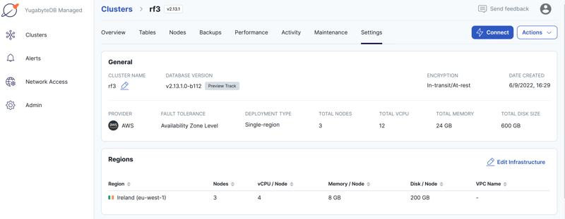
I see the same number of seek() calls as without the filter, and two times more next() calls. The number of seek() look like there are 1000 calls to the tservers. And I can confirm that by logging yb_debug_log_docdb_requests. However, the consequence is not the same as with the Nested Loop because the elapsed time show 60 milliseconds. In this case, where all values are known from the beginning, those many calls are buffered to reduce the remote calls. The time in my single-VM lab is not significant, so lets run it on a real cluster. I provisioned a multi-AZ cluster (where cross-AZ latency is 1 millisecond) in cloud.yugabyte.com to confirm the performance. Here is my cluster in AWS (Ireland):
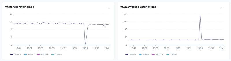
I have run the query using the range sharding (b_pkey) in a loop until 19:25 then created the hash_sharded index b_hkey and ran the query with a hint to use it.
As seen above, the execution time is similar (a few additional milliseconds with hash sharding) and the throughput as well (I'm running from a single session), around 8 SELECTs per seconds:
The internal DocDB operations are different, but the final time is the same. 13 operations per SELECT at average 1.7 millisecond with range sharding. 4 per select with hash sharding, around 8 milliseconds:
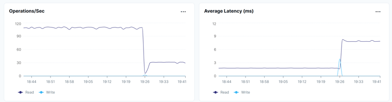
Finally, the way the SQL query decomposed into DocDB calls doesn't change the time and the work done:
Follower reads
On this multi-AZ cluster, I'm also another possible improvement when the query cannot be changed. Nested Loop do too many calls to the tservers. If we can run read-only transaction and accept a small staleness (30 second by default) enabling Follower Reads will reduce the execution time.
Here is my query with Nested Loops:
yugabyte=> explain (costs off, analyze)
           /*+ Leading((a b)) NestLoop(a b) */
           select * from a natural join b where a.x=0;
                                      QUERY PLAN
---------------------------------------------------------------------------------------
 Nested Loop (actual time=4.438..753.609 rows=10000 loops=1)
   ->  Index Only Scan using ax on a (actual time=3.967..4.718 rows=1000 loops=1)
         Index Cond: (x = 0)
         Heap Fetches: 0
   ->  Index Only Scan using b_hkey on b (actual time=0.732..0.737 rows=10 loops=1000)
         Index Cond: ((a1 = a.a1) AND (a2 = a.a2))
         Heap Fetches: 0
 Planning Time: 0.194 ms
 Execution Time: 754.556 ms
(9 rows)
And the same with follower reads:
yugabyte=> set default_transaction_read_only = true;
SET
yugabyte=> set yb_read_from_followers=true;
SET
yugabyte=> show yb_follower_read_staleness_ms;
 yb_follower_read_staleness_ms
-------------------------------
 30000
(1 row)

yugabyte=> explain (costs off, analyze)
           /*+ Leading((a b)) NestLoop(a b) */
           select * from a natural join b where a.x=0;
                                      QUERY PLAN
---------------------------------------------------------------------------------------
 Nested Loop (actual time=4.601..272.716 rows=10000 loops=1)
   ->  Index Only Scan using ax on a (actual time=4.072..4.704 rows=1000 loops=1)
         Index Cond: (x = 0)
         Heap Fetches: 0
   ->  Index Only Scan using b_hkey on b (actual time=0.253..0.257 rows=10 loops=1000)
         Index Cond: ((a1 = a.a1) AND (a2 = a.a2))
         Heap Fetches: 0
 Planning Time: 0.186 ms
 Execution Time: 273.683 ms
(9 rows)
In my example, the execution is x2.5 times faster with follower reads. But I have a small cluster with one node per AZ, which means that follower reads are within the same node. The gain can be less when reading from other nodes in the same AZ. However, Follower Read can help a lot on a multi-region deployment.
Summary
I agree that this technique is a bit cumbersome, but the PostgreSQL compatibility of YugabyteDB makes quite easy. I used psql variables here, but you can do the same from any language, building dynamically the SQL statement with the list. Unfortunately, this has to be a list of literals to be pushed down, and, as far as I know, cannot be done with a subquery. I think it is better to limit the size of the list to avoid memory surprises. In some cases, passing only a range (min/max values) can be sufficient. And don't forget your isolation levels to get repeatable reads between the two queries.


Top comments (0)