As Data Scientists, people tend to think what they do is developing and experimenting with sophisticated and complicated algorithms, and produce state of the art results. This is largely true. It is what a data scientist is mostly proud of and the most innovative and rewarding part. But what people usually don’t see is the sweat they go through to gather, process, and massage the data that leads to the great results. That’s why you can see SQL appears on most of the data scientist position requirements.
What is SPARQL?
There is another query language that could prove very useful in acquiring data from multiple sources and databases, Wikipedia the biggest among them. The query language is called SPARQL. According to Wikipedia:
SPARQL (pronounced “sparkle”, a recursive acronym[2] for SPARQL Protocol and RDF Query Language) is an RDF query language — that is, a semantic query language for databases — able to retrieve and manipulate data stored in Resource Description Framework (RDF) format
Well, this is not a very good definition. It hardly tells you what it can do. To translate it into human-readable language:
SPARQL is a query language similar to SQL in syntax but works on a knowledge graph database like Wikipedia, that allows you to extract knowledge and information by defining a series of filters and constraints.
If this is still too abstract to you, look at the image below:
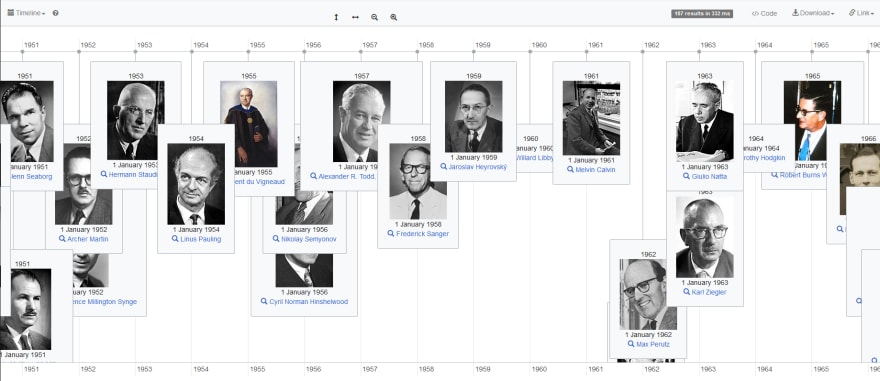 Awarded Chemistry Nobel Prizes
It is a timeline of awarded chemistry Nobel prizes, generated by the WikiData Query Service website, using the code below:
    #Awarded Chemistry Nobel Prizes
    #defaultView:Timeline
    SELECT DISTINCT ?item ?itemLabel ?when (YEAR(?when) as ?date) ?pic
    WHERE {
      ?item p:P166 ?awardStat . # … with an awarded(P166) statement
      ?awardStat ps:P166 wd:Q44585 . # … that has the value Nobel Prize in Chemistry (Q35637)
      ?awardStat pq:P585 ?when . # when did he receive the Nobel prize

    SERVICE wikibase:label { bd:serviceParam wikibase:language "en" . }
    OPTIONAL { ?item wdt:P18 ?pic }
    }
Anyone familiar with SQL will find the above code quite intuitive. I’ll use another example to explain basically how to formulate similar queries to achieve the results you interested in.
Starting Point: Wikipedia Page
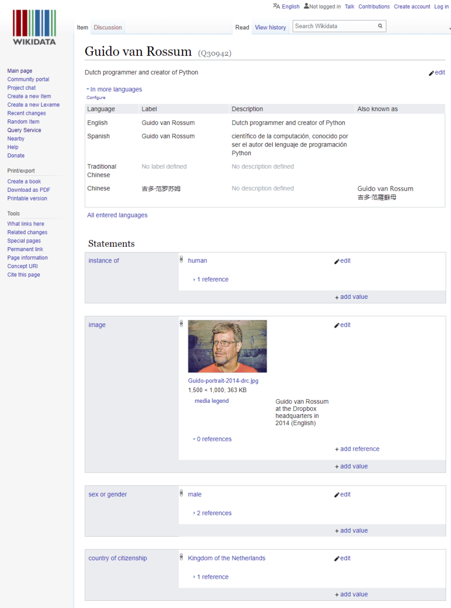
SPARQL works on multiple knowledge graph databases. To know what knowledge graph is, let’s start with something everyone is familiar with: Wikipedia. Wikipedia is the go-to place for most people when they want to research a topic/subject. If you go to Python creator Guido van Rossum’s page, you’ll see a detailed page with all kinds of good information.
Organized Page: WikiData
The problem with this page is it’s not organized. You can search on keywords, but you cannot easily find out the relationship between the information nodes. That’s where the knowledge graph comes into play. The red rectangle on the above page spells “Wikidata Item”, click it will bring you to the knowledge graph view of the same page:
Start the Query
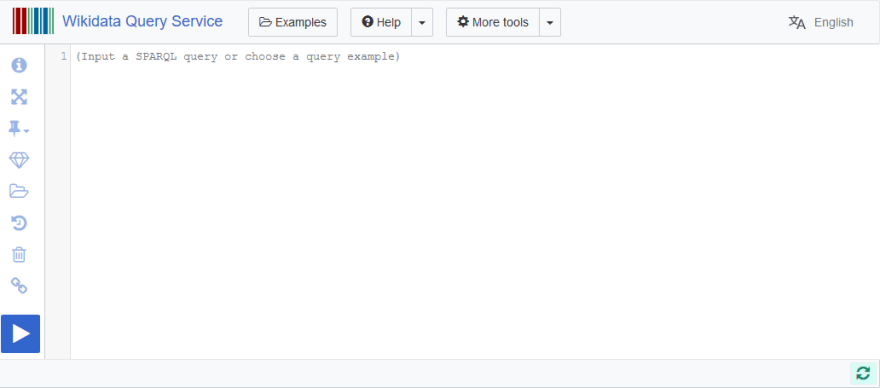
Here we can see all information about Guido is well organized into categories, each category has multiple items. Use SPARQL, you can easily query this information. To do this, Wikipedia provides another page, a user-friendly query service called Wikidata Query Service:
This is where we can experiment with SPARQL. On the WikiData page, we observed that Guido is a programmer (obviously!), now what if we want to know other programmers that have an entry on Wikipedia? Let’s see the SPARQL code:
SELECT ?person

WHERE {

?person wdt:P106 wd:Q5482740 .

}
Here we defined a ?person as the **subject **of interest, this is also what will appear as a column in our query results. Then we specify some constraints with WHERE . The constraints are wdt:P106 need to be wd:Q5482740. What? You say. Let me explain it in more detail. wdt is a prefix of a ‘predicate’ or ‘attribute’ of the subject while wd is the prefix of a value(object in SPARQL terms, but that’s not important) of the attribute. wdt: means I am gonna specify an attribute of the subject here, and wd: means I will specify what the value of this attribute is. So what is P106 and Q5482740 ? These are just a code for the specific attribute and value. P106 stands for ‘occupation’ and Q5482740 stands for ‘programmer’. This line of code means, I want the ?person subject to have an attribute of ‘occupation’ of ‘programmer’. Not that scary anymore, right? You can find these codes easily on the WikiData page mentioned above.
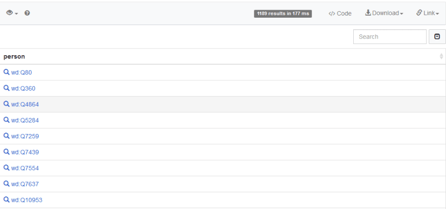
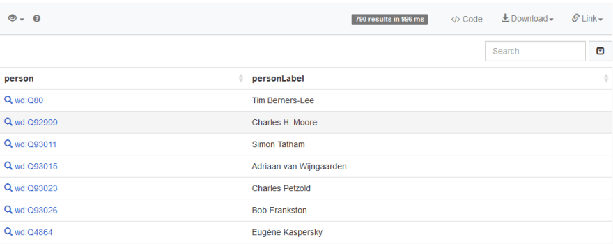
Run the query and you’ll get the following results:
From Code to Name
We got a bunch of person items with different wd:value . If you look closer at the value, they are actually the code for a different person. For example, the first one wd:Q80 is Tim Berners-Lee, the inventor of WWW. This is not intuitive, we want to be able to directly see the names. To do that, we add a WikiData ‘label service’ that helps us translate the code to name, like so:
SELECT ?person ?personLabel

WHERE {

  ?person wdt:P106 wd:Q5482740 .
  ?person rdfs:label ?personLabel .
  FILTER ( LANGMATCHES ( LANG ( ?personLabel ), "fr" ) )

}
Similar syntax, we want the person to have a ‘label’ attribute, and we define a personLabel value variable to hold these values so we can display them in the query results. Also, we added the personLabel into our SELECT phrase so it will be displayed. Please be noted that I also added a FILTER below to only display the French language label, otherwise it will show multiple language labels for one person, which is not what we want:
Narrowing Down
From the above results, we can see that we have some 790 results. This is way too many. Let’s narrow them down to the ones that are ‘somebody’ in the industry. Someone that has an attribute of ‘notable work’:
SELECT ?person ?personLabel ?notableworkLabel

WHERE {

?person wdt:P106 wd:Q5482740 .
  ?person rdfs:label ?personLabel .
  FILTER ( LANGMATCHES ( LANG ( ?personLabel ), "fr" ) )

  ?person wdt:P800 ?notablework .
  ?notablework rdfs:label ?notableworkLabel .
  FILTER ( LANGMATCHES ( LANG ( ?notableworkLabel ), "fr" ) )

}
Again, wdt:P800 means ‘notable work’ attribute, everything else is similar. We then get the following results:
Group Multiple Labels
Now we have only 175 results, with each person’s notable work also listed. But wait, why we have five Richard Stallman? Turns out, Richard has more than one notable work, thus listed multiple times in the results. Let’s fix this by grouping all the notable work into one attribute:
SELECT ?person ?personLabel ( GROUP_CONCAT ( DISTINCT ?notableworkLabel; separator="; " ) AS ?works )

WHERE {

?person wdt:P106 wd:Q5482740 .
  ?person rdfs:label ?personLabel .
  FILTER ( LANGMATCHES ( LANG ( ?personLabel ), "fr" ) )

  ?person wdt:P800 ?notablework .
  ?notablework rdfs:label ?notableworkLabel .
  FILTER ( LANGMATCHES ( LANG ( ?notableworkLabel ), "fr" ) )

}

GROUP BY ?person ?personLabel
Here ‘GROUP BY’ is used. Also, GROUP_CONCAT function is used to concatenate multiple notableworkLabel into a new column works (I will not explain how these functions work, just want to quickly show you what SPARQL can do. Please feel free to Google if you want to know more, there are plenty of tutorial articles and videos out there):
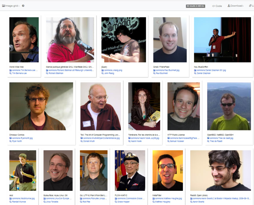
Faces
Now we have a 90 results list, with all the ‘who-is-who’ in the software engineering world. But SPARQL can do more. Let’s add some faces to the names:
SELECT ?person ?personLabel ( GROUP_CONCAT ( DISTINCT ?notableworkLabel; separator="; " ) AS ?works ) ?image

WHERE {

?person wdt:P106 wd:Q5482740 .
  ?person rdfs:label ?personLabel .
  FILTER ( LANGMATCHES ( LANG ( ?personLabel ), "fr" ) )

  ?person wdt:P800 ?notablework .
  ?notablework rdfs:label ?notableworkLabel .
  FILTER ( LANGMATCHES ( LANG ( ?notableworkLabel ), "fr" ) )

  OPTIONAL {?person wdt:P18 ?image}

}

GROUP BY ?person ?personLabel ?image
The same pattern, we just added an OPTIONAL keyword prior since we don’t want to exclude someone if he doesn’t have an image in his profile. We also switch the view into ‘Image Grid’ :
Where are they?
Wow! This is much better. I saw quite some familiar faces! Maybe you wonder where are these guys located? Let’s find out:
#defaultView:ImageGrid

SELECT ?person ?personLabel ( GROUP_CONCAT ( DISTINCT ?notableworkLabel; separator="; " ) AS ?works ) ?image ?countryLabel ?cood

WHERE {
  ?person wdt:P106 wd:Q5482740 .
  ?person rdfs:label ?personLabel .
  FILTER ( LANGMATCHES ( LANG ( ?personLabel ), "fr" ) )

  ?person wdt:P800 ?notablework .
  ?notablework rdfs:label ?notableworkLabel .
  FILTER ( LANGMATCHES ( LANG ( ?notableworkLabel ), "fr" ) )


  OPTIONAL {?person wdt:P18 ?image}

  OPTIONAL {?person wdt:P19 ?country .
           ?country rdfs:label ?countryLabel .
            ?country wdt:P625 ?cood .
            FILTER ( LANGMATCHES ( LANG ( ?countryLabel ), "fr" ) )
           }

}

GROUP BY ?person ?personLabel ?image ?countryLabel ?cood
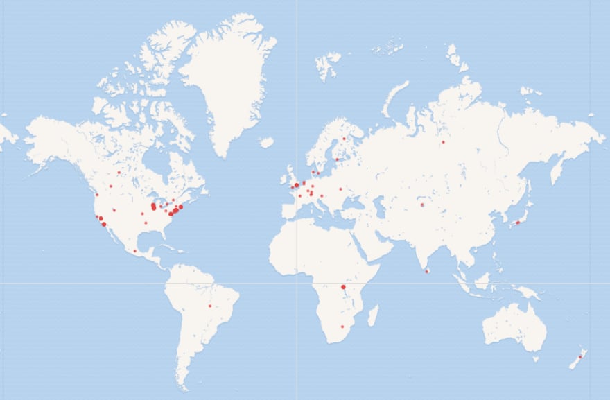
You can decipher the code above yourself maybe. It basically says I want this person to have an attribute of country, put into a variable country, then find out the coordinates of the country and put into a variable cood. With the coordinates, we can activate the ‘map’ view:
We can see we have a lot of them in the US, some in Europe and others scattered around other parts of the world.
More Examples
With a few lines of codes, we figured out the big influencers in the software industry, what they are known of, where they are and how they look. As you can see the potential here is limitless.
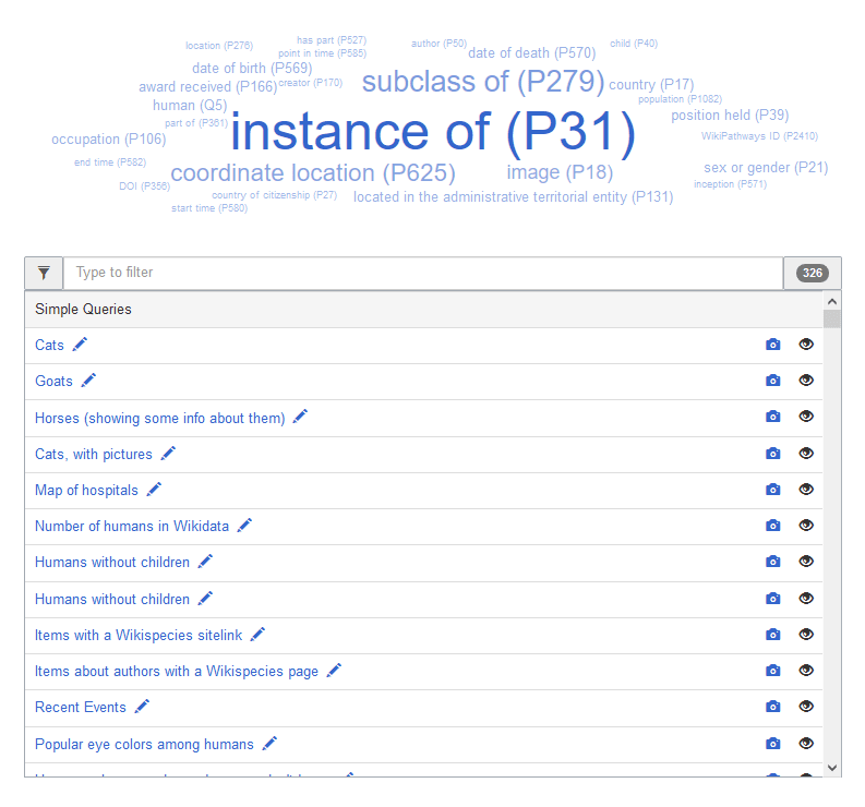
You can click the ‘Example’ button on the WikiData page to find out more fun and interesting examples you can do with it.
As an assignment for this article, can you figure out how to add the ‘date of birth’ attribute and generate a timeline graph like the one at the beginning of this article?
Conclusion
In this article, we used WikiData as a knowledge graph example to introduce SPARQL query language. There are other knowledge graphs out there like DBpedia, etc. This article is by no means a comprehensive tutorial. I just want to introduce the language to more people, so knowledge and information extraction can be done a bit more efficiently.





Top comments (0)