This article gives an introduction to speech signals and its analysis. Also, I have compared with text analysis to see how it different it is from speech.
Speech as compared to text as a medium of communication
Speech is defined as the expression of thoughts and feelings by articulating sounds. Speech is the most natural, intuitive and preferred means of communication by human beings. The perceptual variability of speech exists in the form of various languages, dialects, accents, while the vocabulary of speech is growing day by day. More intricate variability at the speech signal level exists in the form of varying amplitude, duration, pitch, timbre and speaker variability.
Text as a means of communication evolved to store and convey information over long distances. It is the written representation of any speech communication. It is a more simple form of communication and is devoid of the previously mentioned intricate variabilities existing in speech.
The intricate variabilities in speech makes it more complicated to analyse but provides additional information using the tone and amplitude variation.
Representation of speech and text
Speech and text analysis have wide applications in the present world. They have different representations, and many dissimilarities and challenges are encountered in their analysis.
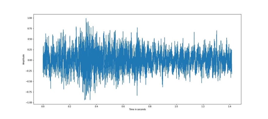
Let us look at a speech signal taken from one utterance of CMU US RMS ARCTIC speech database. Each of the utterances are recorded as a 16 bit signal at a sampling frequency of 16 kHz, which means there are 16000 samples for each second of the signal and each sample has a resolution of 16 bits per sample. Sampling frequency of an audio signal determines the resolution of the audio samples, higher the sampling rate, higher is the resolution of the signal. Speech signal is read from ‘arctic_a0005.wav’ file in the speech database which has a duration of around 1.4 seconds, equivalent to a sequence of 22640 samples, each sample a 16 bit number. The below speech representation is a plot of the speech signal from ‘arctic_a0005.wav’ whose equivalent text is “will we ever forget it” :
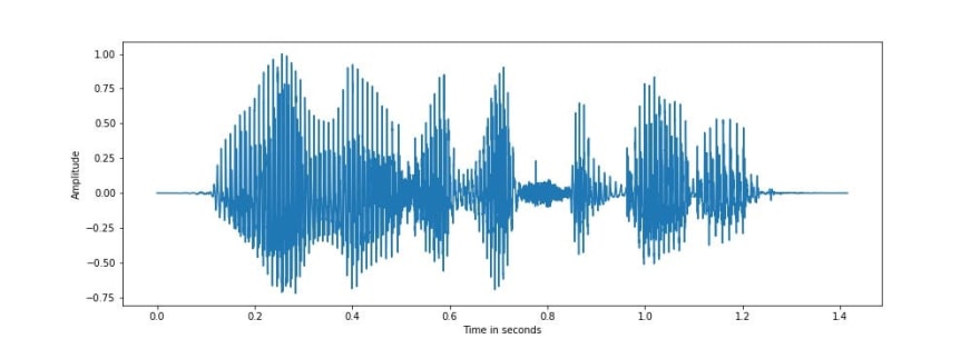
It can be seen from the above figure that speech can be represented as a variation of amplitude with time. The amplitude is normalised such that the maximum value is 1. Speech is basically a sequence of articulate sound units like ‘w’, ‘ih’ known as phonemes. Speech signal can be segmented into a sequence of phonemes and silence/ non-speech segments.
The database also contains the corresponding text transcription for the speech signal both at sentence and phoneme level for each wave file. Below is the representation of a part of the above speech signal showing the phonemes and their corresponding time span.
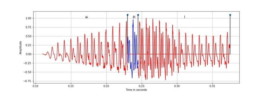
It is seen from the above figure that the phonemes ‘w’, ‘ih’ and ‘l’ are quasi-periodic in nature, and are categorised as voiced phonemes as they are produced by periodic vibration of vocal folds. Further, ‘ih’ is a vowel while ‘w’ and ‘l’ are semi-vowels. Voiced and unvoiced classes are the broad categorisation of speech sounds based on the vibration of vocal cords. The study and classification of different phonemes is called as phonetics.
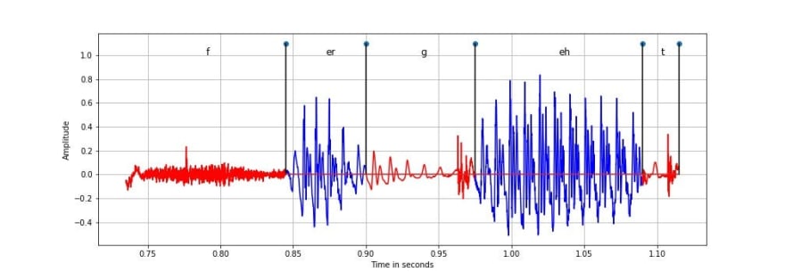
In the above figure we have unvoiced phonemes like ‘f’, ‘g’ and ‘t’ and voiced phonemes like ‘er’ and ‘eh’. Phonemes ‘g’ and ‘t’ are further categorised as stops which is silence followed by a sudden impulse. It can be observed that the voiced component is quasi periodic while unvoiced components are noisy as they are not produced by periodic vibration of vocal folds.
The phonemes can be mapped to the written form of speech using a phoneme to grapheme mapping. Below is the mapping between the text and the corresponding phonemes:
Text: “will we ever forget it”
Phonetic sequence: ‘w’, ‘ih’, ‘l’, ‘w’, ‘iy’, ‘eh’, ‘v’, ‘er’, ‘f’, ‘er’, ‘g’, ‘eh’, ‘t’, ‘ih’, ‘t’
From the above mapping, it can be seen that the word “will” is mapped to the phonemes ‘w’, ‘ih’, ‘l’.
Further we will look at the frame level frequency domain representation of speech, also popularly known as Short-time Fourier transform (STFT) in the speech research community. Spectrogram is a visual representation of the frequency domain representation of sound.
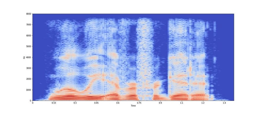
Log scaled spectrogram plotted above is the amplitude of STFT in the log scale. A frame size of 30 ms is chosen which is equivalent to 30 ms x 16 kHz = 480 samples of the speech signal, while frame shift of 7.5 ms is equivalent to 120 samples. The reason behind dividing the speech signal into frames of small duration is that the speech signal is non-stationary and its temporal characteristics change very fast. So, by taking a small frame size, we make an assumption that the speech signal will be stationary and its characteristics will not vary much within the frame. Also, a shorter frame shift is chosen to track the continuity in the speech signal and not miss out any abrupt changes at the edges of the frames. It can be seen from the above plot that frequency domain representation of each frame helps us to analyse speech signal better; as we can easily see the harmonics as parallel red segments in voiced regions and how the amplitude varies for each frequency and frame index. Hence, most of analysis of the speech signal is done in frequency domain. But extraction of temporal information like abrupt changes in the signal (beginning of burst like ‘t’) is better captured in time domain as dividing speech signal into frames discards instantaneous changes in the signal.
We can say that we can get better temporal resolution in the frequency domain by taking a smaller frame size. But there is a tradeoff between resolution in time and frequency domain. Taking a very small frame size will give a higher resolution in time but will give few samples in a single frame and the corresponding Fourier components will have few frequency components. And taking a larger frame size will give lower time resolution but higher frequency resolution due to higher number of samples. So, getting a high resolution both in time and frequency simultaneously is not possible.
It is observed that the y-axis in the log spectrogram plot has frequency upto 8 kHz for a sampling frequency of 16 kHz. This is because, as per Nyquist–Shannon sampling theorem, the maximum frequency which can be observed in a discrete signal is at most half of the sampling frequency which is 8 kHz.
While speech has a lot of variability depending on the environment, speaker, mood and tone of the speaker, text is devoid of all this variability.
The equivalent text is represented as a sequence of alphabets, symbols and spaces as “will we ever forget it”.
Applications of speech analysis
Voice activity detection: Identifying segments in a audio waveform where only speech is present, neglecting the non-speech and silent segments
Speech enhancement: Improving the quality of speech signal by filtering and separating the noise from the speech segments
Speech recognition: Converting the speech signal to text, still its a challenge in different conditions, recognition can be vocabulary dependent or independent
Text to speech: Synthesising natural speech from text, making the speech sound very natural with emotions is challenging
Speaker diarization and speaker recognition: Diarization is segmenting the speech signal into segments belonging to different speakers while speaker recognition is identifying who is speaking at a particular time
Audio source separation: Separating mixed speech signal like speech overlapped with speech from a different speaker or noise
Speech modification: Modifying speech like changing its emotion, tone, converting to speech spoken by a different speaker
Emotional speech classification: Identifying emotion of the speech like happy, angry, sad and anxiety
Keyword spotting: Identifying specific keywords in the whole speech utterance
Applications of text analysis:
Text classification: Classifying the whole text document into various classes, or sequence of words into different classes
Named entity recognition: Identifying people, organisations, place names, certain abbreviations and other entities
Text summarisation: Generating summary from documents
Document clustering: Identifying similar text documents based on similar content
Sentiment analysis: Identifying the mood, emotion, sentiment and opinion from the text
Challenges in speech and noise analysis:
All the above applications of speech and noise analysis are quite challenging to solve. External factors which further complicate speech and noise analysis are various kinds of noise incurred along with the speech and text. Various signal processing, neuroscience based methods, supervised and unsupervised machine learning techniques are explored to solve the same. Due to the unstructured nature of speech signals, deep learning based methods have shown success for various applications.
Noise in speech and text :
Noise is any unwanted signal distorting the original signal. Adding noise to speech vs adding noise to text is very different.
Given a speech signal with amplitude s[n], where n is the sample index, noise is any other signal, w[n] which interferes with the speech. The noisy speech signal u[n] can be seen as:
u[n]=s[n] + w[n]
In the above case, the noise is additive in nature, which is the most simple case. Noise can also incur in a convolutional form such as reverberation, amplitude clipping and other non-linear distortions of the speech signal.

The above plot is of factory1 noise both in time and frequency domain which is taken from the NOISEX92 database. The above noise samples are resampled to the same sampling rate of speech samples, 16 kHz as we are adding speech to noise and both should have same sampling rate.
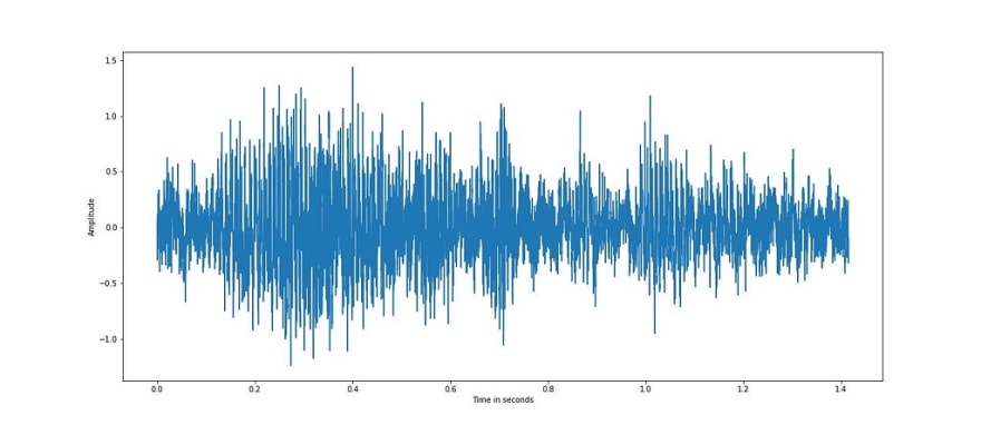
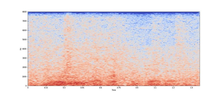
The above plot is of noisy speech both in time and frequency domain. Noise in a speech signal modifies the whole signal and it is difficult to analyse and extract speech segments. Various speech enhancements algorithms exist to reduce the noise component and improve the intelligibility of speech.
Given text sentence, noise can incur in the form of misspelt and missing words which may either change the meaning of the sentence or create a meaningless sentence. For example:
Original text sentence: ‘will we ever forget it’
Noisy text sentence : ‘will we never forget it’
In the above noisy text, noise incurs in the form of the word ‘ever’ changed to ‘never’, which changes the meaning of the sentence.
Another form of noisy text: ‘will we never forggt it’
In the above noisy text, noise incurs in the form of the word ‘forget’ changed to ‘forggt’, which makes the sentence meaningless due to the misspelt word ‘forggt’.
So, it can be seen that adding noise to speech distorts the whole signal while in text distortion is discrete like missing a character/word or mispelling.
Illustration of speech analysis
We will now illustrate an important speech analysis technique. A recording of any audio signal in general contains lot of silence regions and we may be interested only in the segments where speech is present. This is useful to extract speech segments from the signal containing long silence regions automatically as silence regions do not convey any information. These speech segments can be further analysed for various applications like speech recognition, speaker and emotion classification.
Hence, silence detection is an important pre-processing step in most of the speech applications.
Given a speech signal s[n], silence regions can be detected by comparing the relative energy of segments within short durations. We take a frame size of 20 ms and calculate the short term energy signal, e[n] as sum of square of s[m] where m is within +/-10 ms (in samples) of n . The frame size is chosen depending on how much temporal change in energy of the speech signal we want to detect. A short frame size is able to detect abrupt change in energy but may give many alternating frames of silence segments due to inherent silence parts in some phonemes like bursts and in between words.
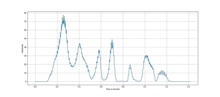
It is seen from the above plot that the short term energy of the speech signal varies abruptly and a relative threshold can be used to detect silence regions.
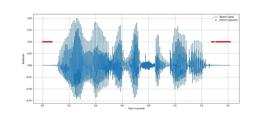
The above plot shows the silence regions highlighted in red by using a threshold of 0.01% of the average short term energy of the speech signal. The threshold is chosen based on observation of the variation of short term energy in the speech signal.
One challenge in silence detection is in case the speech signal is noisy, then the relative energy in silence regions of speech will also be high. This can be solved by seeing the variation of short term energy of lowpass filtered speech signal in case the noise has predominantly high frequency components.
Demo of the simulations done in the present article can be found at Github and NBViewer .
Hope you found this article and demo useful. I will try to add more insights on the analysis of speech signal in the upcoming articles.
About the author
I am a Data Scientist at Belong.co and have finished my PhD from the Indian Institute of Science Bangalore, India.


Top comments (0)