Can water stress be accurately modeled using Remote sensing data?

_I created a irrigation recommendation model that can inform farmers when to irrigate and for how long based on water stress

https://colab.research.google.com/drive/1qrSgb5Wn4oW2_Vvnv4AHTumRUi6R_9NB#scrollTo=Z7ZX8hj7FapM

With increasing temperatures and extreme rainfall fluctuations, climate change is causing harsher conditions for growing crops. Farming is becoming increasingly difficult as farmers struggle to produce enough food to feed a growing population. As a result, agriculture stands to gain a great deal from data driven models to help inform crop production.
Irrigation is a critical input for agricultural crop production globally. 70% of the world's fresh water is used for irrigation. However, irrigation increases farmers' production costs. At the same time, increased drought events have led to water stress. Water stress from drought will have major impacts on biomass, yield, and quality. However, drought stress can be alleviated with proper irrigation. Thus, having models to quantify water stress in plants can inform farmers on irrigation needs for gains at harvest and reduce inputs to fields. This can save thousands of gallons of water, reduce the production cost for farmers, and protect ecosystems.

I tried to solve the problem of whether it is possible to accurately model crop water stress with remote sensing technology deployed throughout a growing season at the level of a crop's growth. Climate and plant-derived parameters sampled from remote-sensed data sources can be utilized to develop a model to predict plant water stress. We will aim to create a model using remote sensed, in field measurements to determine whether a corn crop is undergoing water stress at a point in time in a growing season for a corn crop. Our goal was to be able to create a model which can take in field specific remote sensed values and predict with a strong degree of accuracy whether the crop in the field is water stressed using the methodology laid out in the Dejonge paper on CWSI. Ultimately, I built out a model to see how close we could get to being able to create the conditions where someone could view the data with strong confidence to make an irrigation decision. The implications of being able to do this are to provide growers with the tools to irrigate more efficiently, to save natural resources, to reduce equipment and labor costs, and to obtain the best outcomes that they can given their climatic conditions.

DATA****
I. Our data source - Arable/UNL partnership; the treatments; the experiment set up; the variables we had available and the ones we didn't have available (soil moisture)
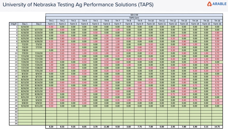
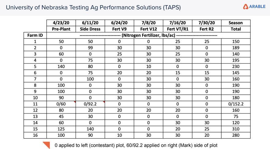
Our data comes from a research site set up at the University of Nebraska-Lincoln. The plots set up were part of the TAPS (Testing Agricultural Performance Solutions) program. In one of their sites they broke down a field into 16 blocks of Pioneer 1197 AMT corn. Each of the 16 blocks received varying rates of irrigation amounts via subsurface drip tape. They also received varying amounts of nitrogen fertilizer. The initial planting date was 5/1/20 with a seed density of 34k per acre. Data was collected over one growing season in all plots. Our study utilizes data from 4 of these plots. The most and least irrigated plots and 2 plots around the first and third quartile were chosen to study a range of irrigation.

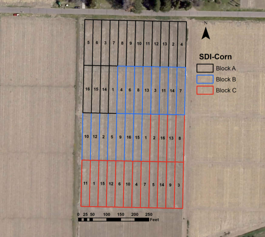
Our research focused on the different treatments of the subblocks of block B.

Within each of the 16 blocks set out in this study 2 Arable Mark II sensors were deployed. These devices collect 40+ continuous data streams including the ones we used for quantifying the water stress of each block. They report data once in hourly intervals for most climatic measurements. The measurements that were most relevant that were collected by the Marks within the individual sub blocks were the precipitation amounts, evapotranspiration, canopy temperature, air temperature, vapor pressure deficit, and solar radiation. On board each sensor is a 7-band spectrometer that can be used for measuring crop spectral indices such as NDVI and Chlorophyll index. These measurements are taken once daily at solar noon. We were provided the data on the different irrigation amounts and fertilizer amounts by our contact at the University of Nebraska.

The Mark sensors have the ability to integrate with soil moisture probes; however, the 2020 season did not have soil moisture data that was simultaneously collected at these sites. In adjacent fields in the study there were other soil moisture probes though we were not able to access that data nor were we able to consider the effects of soil type at all in our research. In the Dejonge paper, soil water potential was used as part of the baseline to quantify water stress at different points in the season. They also included the expected root zone at different parts of the crop’s phenology.

Data cleaning and analysis was done in python. Replicates from each plot were averaged
across all measurements to combine data frames. Irrigation and nitrogen inputs were added based on plot treatments. Total season irrigation and nitrogen inputs were also calculated. Data was trimmed to begin based on the latest start date found in the data and end at harvest. To be able to integrate canopy temp, hourly data was added to daily values at 1200 local device time which will be around the daily temp peak. Finally, crop water stress index was calculated for daily values with a baseline for full irrigation. Once all datasets were built and further features defined, all missing values were filled with the mean of the variable for each data frame. 
Once all features are pulled into the data frame from Mark sensors, further data cleaning allows for the creation of daily water input, crop water demand, and CWSI. Water input is calculated as a simple sum of the
rainfall and irrigation of a given day (in mm). The crop water demand is defined as the daily water input minus evapotranspiration. The formula for CWSI was given by Dejonge et al as the difference in measured canopy and air temp minus the lower limit of difference over the upper limit minus the lower limit, eq. 1
Eq. 1: CWSI = (Tc -Ta-dTLL)/(dTUL-dTLL)   
Where Tc is the canopy temperature of a given plot, Ta is the air temperature, dTLL is the theoretical upper limit difference as defined by a well watered crop, and dTUL is the upper limit of difference recommended to be 5. 
Each plot that we studied(plots 3, 5, 11, and 16) were run through both the linear and the logistic regressions. For each plot we used the train, test, split function from Pythons scikit-learn library. In order to create the logistic regression we created an “is_water_stress” binary in order to model if on a given day the crop was stressed or not
 
Results and Discussion
Exploratory Analysis

We began our approach to determine which model to use and which features to include in it by running a thorough exploratory analysis that looked at some of the individual variables that were collected by the Arable Marks and how they correlated with one another. We compared these features across the different plots that were studied 

Plot 16 was our most irrigated plot. 

Plot 11 was the plot that received no irrigation treatments. The water inputs shown in this chart are purely representative of precipitation. Compared to plot 16 at the end of the season in Septemer, its NDVI was 0.2 less than that of plot 16 indicating that water stress had some negative effect on canopy biomass, at least later in the season. 

We also tried to observe the effects of Nitrogen on the NDVI readings of the multiple plots. Interestingly, we couldn't find a strong correlation between the amount of nitrogen added and NDVI. We also weren’t able to see a strong relationship between the time that nitrogen was added and the resulting NDVI

Plot 3 had stepwise applications of nitrogen. Our “n_total” feature was a running sum of the nitrogen applied over the course of the growing season. 

Plot 11 had all of its nitrogen applied at the start of the season yet it experienced a similar growth curve as Plot 3. 

The last thing we did before beginning modeling was examining how certain features were or were not correlated with one another. Displayed below is our output of a correlation heat map for plots 5 and 11

As to be expected, the features with the highest correlation with our CWSI are below (canopy temperature) and vapor_pressure_deficit(VPD).

II. Linear Regression
We ran two kinds of linear regressions: a simple one where we observed the efficacy of using individual predictor variables for our crop water stress index and a multiple linear regression where we added in several feature combinations to observe the predicted outcomes. 

In our simple linear regression we used Tbelow (canopy temperature) as our independent variable to our CWSI dependent variable. In the figure below one can see that there is a positive linear relationship between the two. 

After we fit the model we ran a simple prediction based on when our canopy temperature varied throughout the growing season. We tested on 10C and 30C and our model returned a 39% chance of water stress and an 87% chance respectively. 

Before building our multiple linear regression we defined a set of features and plotted them against CWSI. In the figure below we display plot 11 (least irrigated) and plot 16 (most irrigated).

Comparing our least watered plot (11, top) to the most watered plot (16, bottom).

Next, after fitting our model with the features that we chose, we displayed the coefficients of each of the individual features. We saw that Tbelow had the most predictive power and the highest positive coefficient. 

We then re-ran our model using the train, test, split function in scikitlearn in order to evaluate our models performance with the RMSE and MSE. 

The RMSE was low upon adding in 4 features. It is worth noting that of the features we used, max_temp, tbelow, and air_temp are highly correlated.
Lastly we compare the MSE of our trained data to that of our test set and see that we receive similar values. We saw that the MSE of our trained data set was .047 while our test data was .05 indicating a similarity in accuracy. To make this analysis more robust it would be instructive to try to run a similar analysis across a similarly set up experiment in another region to evaluate the performance of our model. 

Logistic Regression Steps


1. Converting  CWSI to a categorical variable (0 = nonstressed, 1=stressed) Our second model was an attempt to create a logistic regression model with the idea that it would also be useful for providing a simpler binary recommendation to irrigators as to when their crops are water stressed or not. We began by converting our CWSI into a categorical variable called is_water_stressed where 0= non-stressed and 1 = stressed. 
2. Scatter plot including the regression line(left) and with predicted values(right) Before creating our logistic regression we wanted to show our linear regression through the is_water_stressed variable: 

Next after creating our predicted class of water stress (is_water_stress_pred_class), we plot that line against is_water stress. We created our predicted class based on the observation that the midpoint of our regression line was approximately .6 CWSI. This showed that our data was roughly split in half. 

1. Using the logistic regression to predict the probability a given row is 0 or 1
   Our third step was to use the logistic regression to observe if a given day in our data set had a high probability of being water stressed or not. We ran the code below to observe the likelihood that there was water stress between the 40-50 days of the growing season as this is typically a sensitive period in corn phenology. 

2. Prediction given that Tbelow is a certain temperature and plotting the logistic regressions with a predicted Sigmoid curve

Next we plotted the probability of a given row in the top plot and then used the logistic regression to show the likelihood that the corn plant would be water stressed at a given reading of canopy temperature. As one would expect, higher canopy temperatures significantly increase the likelihood of water stress. The left column is the likelihood of zero while the right is the likelihood of 1.  

1. Log Odds what was our confidence in our ability to predict

Lastly, we convert the odds given to us by the logistic regression to a probability. In the example below we display the log odds of tbelow at 30C and convert those odds to a probability. The result is that we are told there is a 76% chance there is crop water stress at 30C. We also calculated an accuracy score of 92% on our model after splitting the data into training and testing sets. This number could perhaps be even further enhanced if more features were added to the logistic equation.