
Summary: This article explains how to build and modify a simple fire model, and explores two popular methods to simulate fire spread—cellular automata and wave propagation. This article was originally published on Triplebyte's blog.
It’s Fire Season
In July, the Western United States enters the core of the fire season. Many parts of the country are experiencing below-average precipitation and above-average temperatures—creating hot, dry conditions that are ideal for wildfires.
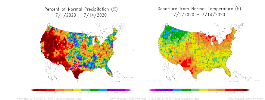
NOAA Regional Climate Centers: Generated at HPRCC using provisional data.
Mathematical models of fire behavior, and the calculation systems based on them, are an important part of fire mitigation. Fire models can help determine where a fire is likely to start, how quickly it will spread (and in what direction), and how much heat it will generate; these important clues can save lives and substantially curb financial losses.
Modeling Fire Growth: Cellular Automata
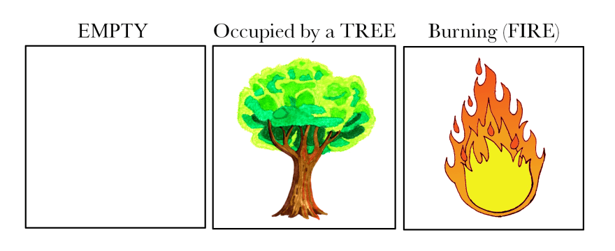
A simple cellular automaton forest fire model consists of a grid of cells, and each cell can be in one of three states:
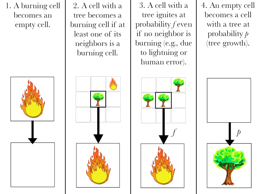
At each time step, the state of each cell on the grid is determined by four rules that the model carries out simultaneously:
A Cellular Forest Fire Model in Python
These four fire model rules are implemented by the iterate function of a cellular automaton model created by Christian Hill1.
# This function iterates the forest fire model according to the 4 fire model rules.
# X is the current state of the forest and X1 is the future state.
def iterate(X):

    # RULE 1 ("A burning cell becomes an empty cell") is handled by
    # setting X1 to 0 initially and having no rules that update FIRE cells.
    X1 = np.zeros((ny, nx))
    for ix in range(1,nx-1):
         for iy in range(1,ny-1):

            # RULE 4 ("An empty cell becomes a cell with a tree at probability p")
            if X[iy,ix] == EMPTY and np.random.random() <= p:
                 X1[iy,ix] = TREE

            # RULE 2 ("A cell with a tree becomes a burning cell if at least one
            # of its neighbors is a burning cell.")
            if X[iy,ix] == TREE:
                 X1[iy,ix] = TREE
                 for dx,dy in neighborhood:
                     if X[iy+dy,ix+dx] == FIRE:
                         X1[iy,ix] = FIRE
                         break

                 # RULE 3 ("A cell with a tree ignites at probability f even if
                 # none of its neighbors are burning").
                 else:
                     if np.random.random() <= f:
                         X1[iy,ix] = FIRE
         return X1
Modifying the Model
Some simple modifications to the code can add other features to the model that influence fire spread. For example, to add water bodies—which can block fire spread, I first defined a new cell state (WATER) and expanded the color list and bounds accordingly:
EMPTY, TREE, FIRE, WATER = 0, 1, 2, 3
colors_list = [(0.2,0,0), (0,0.5,0), (1,0,0), 'orange', 'blue']
cmap = colors.ListedColormap(colors_list)
bounds = [0,1,2,3,4]
norm = colors.BoundaryNorm(bounds, cmap.N)
Then, I added another rule to the iterate function, which simply ensures that WATER cells remain WATER cells.
def iterate(X):
    X1 = np.zeros((ny, nx))
    for ix in range(1,nx-1):
         for iy in range(1,ny-1):
            if X[iy,ix] == WATER:
                 X1[iy,ix] = WATER
            if X[iy,ix] == EMPTY and np.random.random() <= p:
                 X1[iy,ix] = TREE
            if X[iy,ix] == TREE:
                 X1[iy,ix] = TREE
                 for dx,dy in neighborhood:
                     if X[iy+dy,ix+dx] == FIRE:
                         X1[iy,ix] = FIRE
                         break
                 else:
                     if np.random.random() <= f:
                         X1[iy,ix] = FIRE
         return X1
Finally, I defined the boundaries of the water bodies (in this case, four vertical “streams”).
X[10:90, 10:15] = WATER
X[10:90, 40:45] = WATER
X[10:90, 60:65] = WATER
X[10:90, 80:85] = WATER
These adjustments produce a model that shows how fire growth is restricted by water:
Notably, fire can sometimes “jump” over barriers—a behavior called spotting that creates trouble for fire modelers and responders alike.
The original model can also be modified to include wind, which can dramatically affect fire spread. To achieve this, I first modified the original neighborhood (commented out below), such that NY and NX respectively represent the first and second coordinates of the original neighborhood.
# neighborhood = ((-1,-1), (-1,0), (-1,1), (0,-1), (0, 1), (1,-1), (1,0), (1,1))
# NY and NX are now neighborhood
NY=([-1,-1,-1,0,0,1,1,1])
NX=([-1,0,1,-1,1,-1,0,1])
Just below NY and NX, I defined NZ, which represents wind. Each value in NZ corresponds to one of the coordinates in neighborhood (NY and NX). If at least one of the index values in a neighbor-specifying pair of NY, NX is negative, the corresponding NZ value is 0.1. Otherwise, NZ is 1. As a concrete example, the first value of both NY and NX is -1, so this first pair of coordinates corresponds to the neighbor at (-1,-1). Thus, the NZ value corresponding to this pair is 0.1. This modification ends up biasing fire spread in the direction that wind is blowing, as I explain shortly.
NZ=([.1,.1,.1,.1,1,.1,1,1])
The final step is to modify the iterate function to check all neighboring cells. If a neighbor is on fire AND a randomly generated number is less than the neighbor's NZ value (0.1 or 1), the cell catches on fire. Since the random number is a float >0 and <1, when NZ = 1, the random number will always be smaller and the cell will burn. Similarly, 0.1 is below most random numbers generated. This biases fire spread with wind direction.
def iterate(X):
    X1 = np.zeros((ny, nx))
    for ix in range(1,nx-1):
         for iy in range(1,ny-1):
            if X[iy,ix] == EMPTY and np.random.random() <= p:
                 X1[iy,ix] = TREE
            if X[iy,ix] == TREE:
                 X1[iy,ix] = TREE
                 # Check all neighboring cells.
                 for i in range(0,7):
                    # Bias fire spread in the direction of wind.
                    if X[iy+NY[i],ix+NX[i]] == FIRE and np.random.random()<=NZ[i]:
                        X1[iy,ix] = FIRE
                         break
                 else:
                     if np.random.random() <= f:
                         X1[iy,ix] = FIRE
         return X1
This example code produces a fire model with wind blowing uniformly from the southeast.
Modeling Fire Growth: Wave Propagation
Cellular models, like the one depicted above, simulate fire spread as a contagion process in which fire spreads between cells. One of the major shortcomings of this method is that the use of a gridded landscape distorts fire geometry, although there are methods to help mitigate this (e.g., increasing the number of neighbor cells).
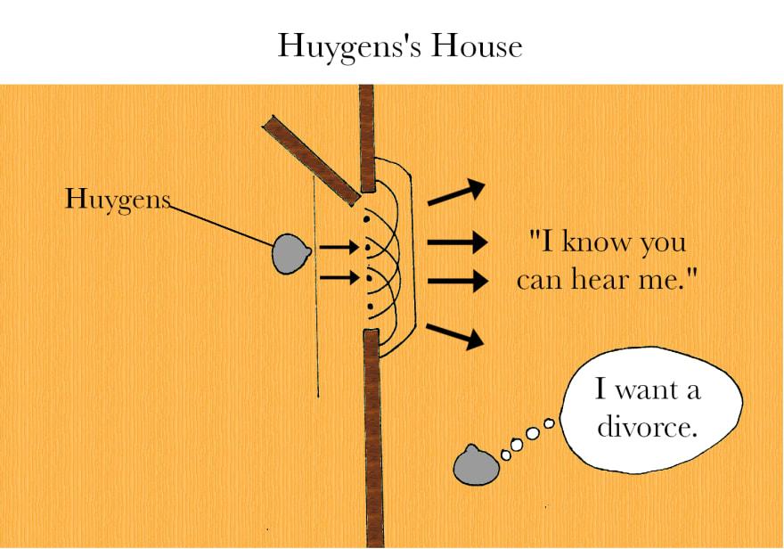
Today, some of the most widely used fire simulators (e.g., FARSITE, Prometheus) are based on Huygens principle of wave propagation. Huygens principle was originally proposed to describe traveling light waves, and also explains how sound waves can travel around corners. The crux of Huygens principle is that every point on the edge of a wave-front can be an independent source of secondary wavelets that propagate (i.e., spread) the wave.
Although Huygens studied light (not sound) and never married, this is what I imagine:
Wave propagation models simulate fire as an elliptical wave that spreads via smaller secondary elliptical fire wavelets on the fire front. At each time step, the model uses information about the fire environment to define the shape, direction, and size (spread rate) of each wavelet. Shape and direction are determined by the wind-slope vector, while size is determined by fuel conditions.
The new wave-front is the surface tangential to all the secondary wavelets. In other words, the small ellipses form a kind of envelope around the original fire perimeter, and the outer edge of this envelope is the new fire front.
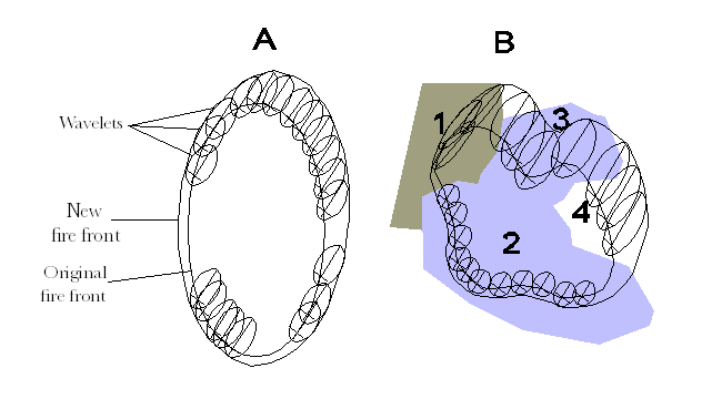
Huygen’s principle in the context of fire spread2. Wind is uniform and traveling from the southwest. A) Fire spread across a landscape with homogeneous fuel sources. B) Fire spread across a mosaic landscape with four different fuel types and wind speeds, which change the size and shape of the wavelets.
Yes, Fire Modeling Is Considerably More Complicated Than This
While cellular automaton and wave propagation models are an essential part of many fire growth simulators, in real-world applications, they become a relatively minor component of a complex simulation process that also incorporates many other models.
These additional models capture factors related to weather, fuel type (fuel is anything that can burn), and topography, which greatly influence fire growth. Additionally, “fires create their own weather,” altering humidity and other aspects of their surrounding environment; this poses a formidable challenge for fire modelers.
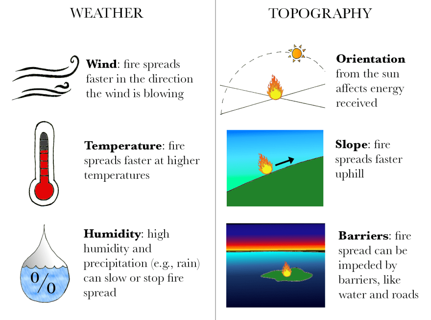
Select examples of weather- and topography-related factors that influence fire growth. These variables are often incorporated in fire growth simulators.
Consider FARSITE (now part of the FlamMap fire mapping and analysis system)—a prominent fire simulator used by the U.S. Forest Service, the National Park Service, and other state and federal agencies.
FARSITE implements Huygens principle using a set of differential equations developed by G.D. Richards in 1990. However, as the table below illustrates, FARSITE also incorporates many other models—as well as several geospatial data layers—to simulate fire growth. Richards’s equations are only used for a single step of the surface fire calculations and a single step of the crown fire calculations.
Models and Geospatial Data Layers Used by FlamMap/FARSITE
| Model | Geospatial data layers for landscape |
|---|---|
| Surface fire spread (Rothermel, 1972) | Topographic (elevation, slope, aspect) |
| Crown fire initiation (Van Wagner, 1977) | Fire behavior fuel models |
| Crown fire spread (Rothermel, 1991) | Forest canopy cover |
| Spotting (Albini, 1979) | Forest canopy height |
| Crown fire calculation (Finney, 1998; Scott and Reinhardt, 2001) | Forest canopy base height |
| Dead fuel moisture (Nelson, 2000) | Forest canopy bulk density |
Fire Modeling Is a Balancing Act
Fire modeling requires tradeoffs among accuracy, data availability, and speed. For real-time responses to fire, speed is critical—yet the most physically complex models are impossible to solve faster than real time. As University of Denver researcher Jan Mandel articulated3:
“The cost of added physical complexity is a corresponding increase in computational cost, so much so that a full three-dimensional explicit treatment of combustion in wildland fuels by direct numerical simulation (DNS) at scales relevant for atmospheric modeling does not exist, is beyond current supercomputers, and does not currently make sense to do because of the limited skill of weather models at spatial resolution under 1 km.”
Notably, there are many types of fire behavior models, and these models can be classified based on the types of equations they use, the variables they study, and the physical systems they represent. For the interested reader, the appendix includes a breakdown of the different model classifications.
→ Coding Challenge
Can you build your own model (e.g., a cellular automaton) to simulate fire spread?
What additional factors can you add to your model?
How do you implement them?
Let me know your thoughts in the comments section!
Triplebyte helps engineers assess and showcase their technical skills and connects them with great opportunities. You can get started here.

Top comments (0)