Training a DATASET Using Linear Regression(An ML technique)

Few days back when I was doing a DS course from uaceit.com ,I learned making my very first data science project on Jupyter Notebook using an effective ML algorithm i.e. Linear Regression. I learnt understanding data and how we can relate it to get better and desired outcomes. Linear Regression can be defined as "An approach that models a change in 1 or more predictor variables(say x) that produces a linear change in the response variable(y)"

Lets get started step by step from scratch

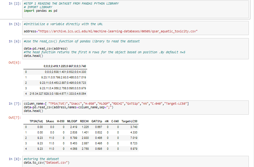
STEP 1 : READING AND ARRANGING DATASET IN PROPER FORMAT

In the 1st step ,I imported pandas library to read dataset with its read.csv() function. The dataset is taken as a link in the address variable. Since the data was raw containing unnamed & unseparated columns ,So it was converted in a readable form. Then stored as Dataset.csv onto my local machine.

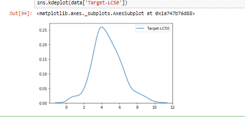
STEP 2: MAKING EXPLORATORY ANALYSIS ON DATA

EDA generally called as Exploratory Data Analysis is a kind of statistical study that is done on data sets to figure out main characteristics and perform hypothesis as required. For that ,we require data visualization library i.e. seaborn to understand the relationship between the different data points/predictors. Info() and describe() functions were used to see where the distribution points lie and the range of the dataset. Since the graph showed symmetrical sign it is observed that the predictors are linearly related with the target variable.

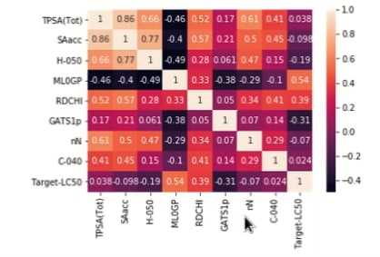
STEP 3: ANALYZING THE CO RELATION BETWEEN VALUES IN A DATASET

To visualize co relation values(from -1 to 1) between predictor and target variable we use heat map() function and corr() function of our data frame to see results.
1 means =>perfect positive linear relationship
-1 means =>perfect negative linear relationship
0 means =>no relationship at all

Consider the last row for better understanding , MLDGP shares the highest positive linear relationship with target variable(0.54) and GATS1p shares the highest negative linear relationship (-0.31)

STEP 4: MODELLING DATASET USING LINEAR REGRESSION

For training and modelling dataset, we will use sklearn python library. We will import StandardScaler () and train_test_split() function from preprocessing and model_selection sub modules of sklearn.

The dataset is divided into 2 parts for training:

X => for displaying the feature variables(independent)

Y => for displaying the response variable(dependent)

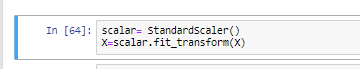
Here, another important concept that needs to be understand is of Scaling .We use the feature scaling technique to standardize the independent variables present in a dataset to a fixed range of minimum and maximum values of 0 to 1.This is done using StandardScaler() function.

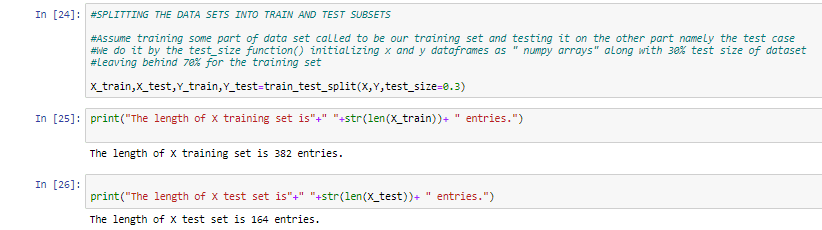
Moreover, the train_test_split() will divide the dataset into two subsets 70% for training and 30% for testing model.

After that, we will apply LinearRegression() method from model selection sub module. The fit method takes 2 arguments for training(input and output) as supervised learning gives predictions on mapping input to output based on randomly organized training sets. We will then apply predict() method for our model to make predictions.

By checking residuals i.e. difference between the observed y-value (from scatter plot) and the predicted y-value (from regression equation line),we will see how appropriate our model and assumptions are .

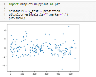
Since, residuals are randomly placed, above and below x-axis(regression line), it is confirmed that our model is Linear Appropriate. This means that a residual may have a positive, negative or zero values.

A linear regression requires residuals to be normally distributed with a mean of 0. Residuals have the same distribution for all values of the explanatory variables. But here we see that our distributed values differ means that the model is biased and we need to revise the model. Problems like overfitting or multi collinearity limits the effectiveness of this algorithm.

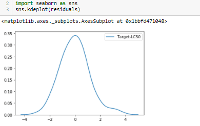
Each time the model is fitted ,it trains a random subset and gives a different accuracy score. The model is able to predict only 40 to 60 % of the target variable which is quite low. In short, the fact that the residuals were not equal to 0 has affected the accuracy rate of the model .You can find the code link at the end of the blog.

One way to address the problem is simply removing those data points which are too distant from the mean of data or we can increase the complexity by adding the number of predictors into dataset.

Other algorithms like KNN-regression, LASSO or Ridge Regression can also be fitted on the model as alternatives to apply regularization to the dataset and improves its accuracy. To learn more about this technique you can follow the links below.

Until then stay connected for new data insight stories!

Have a Good Day :)

Source:

Project:-->https://uaceit.com/courses/your-first-data-science-project/ &

-->https://datatofish.com/multiple-linear-regression-python/

Linear Regression: https://en.wikipedia.org/wiki/Linear_regression

GITHUB repo: https://github.com/ToobaAhmedAlvi/1stDSproject