
Rule-based Sentiment Analysis Using Python and R
Overview
Why Sentiment Analysis?
NLP is subfield of linguistic, computer science and artificial intelligence (wiki), and you could spend years studying it.
However, I wanted a quick dive to a get an intuition for how NLP works, and we'll do that via sentiment analysis, categorizing text by their polarity.
We can't help but feel motivated to see insights about our own social media post, so we'll turn to a well known platform.
How well does Facebook know us?
To find out, I downloaded 14 years of posts to apply text and sentiment analysis. We'l use Python to read and parse json data from Facebook.
We'll perform tasks such as tokenization and normalization aided by Python's Natural Language Toolkit, NLTK. Then, we'll use the Vader module (Hutto & Gilbert, 2014) for rule-based (lexicon) sentiment analysis.
Finally, we'll transition our work flow to R and the tidyverse for data manipulation and visualization.
Getting Data
First, you'll need to download your own Facebook data by following: Setting & Privacy > Setting > Your Facebook Information > Download Your Information > (select) Posts.
Below, I named my file your_posts_1.json, but you can change this.
We'll use Python's json module read in data. We can get a feel for the data with type and len.
import json

# load json into python, assign to 'data'
with open('your_posts_1.json') as file:
    data = json.load(file)

type(data)     # a list
type(data[0])  # first object in the list: a dictionary
len(data)      # my list contains 2166 dictionaries
Here are the Python libraries we use in this post:
import pandas as pd
from nltk.sentiment.vader import SentimentIntensityAnalyzer
from nltk.stem import LancasterStemmer, WordNetLemmatizer      # OPTIONAL (more relevant for individual words)
from nltk.corpus import stopwords
from nltk.probability import FreqDist
import re
import unicodedata
import nltk
import json
import inflect
import matplotlib.pyplot as plt
Natural Language Tookkit is a popular Python platform for working with human language data. While it has over 50 lexical resources, we'll use the Vader Sentiment Lexicon, that is specifically attuned to sentiments expressed in social media.
Regex (regular expressions) will be used to remove punctuation.
Unicode Database will be used to remove non-ASCII characters.
JSON module helps us to read in json from Facebook.
Inflect helps us to convert numbers to words.
Pandas is a powerful data manipulation and data analysis tool for when we save our text data into a data frame and write to csv.
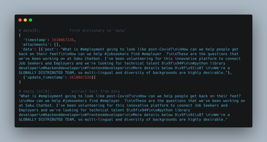
After we have our data, we'll dig through to get actual text data (our posts).
We'll store this in a list.
Note: the data key occasionally returns an empty array and we want to skip over those by checking if len(v) > 0.
# create empty list
empty_lst = []

# multiple nested loops to store all post in empty list
for dct in data:
    for k, v in dct.items():
        if k == 'data':
            if len(v) > 0:
                for k_i, v_i in vee[0].items():
                    if k_i == 'post':
                        empty_lst.append(v_i)

print("This is the empty list: ", empty_lst)
print("\nLength of list: ", len(empty_lst))
We now have a list of strings.
Tokenization
We'll loop through our list of strings (empty_lst) to tokenize each sentence with nltk.sent_tokenize(). We want to split the text into individual sentences.

This yields a list of list, which we'll flatten:
# - list of list, len: 1762 (each list contain sentences)
nested_sent_token = [nltk.sent_tokenize(lst) for lst in empty_lst]

# flatten list, len: 3241
flat_sent_token = [item for sublist in nested_sent_token for item in sublist]
print("Flatten sentence token: ", len(flat_sent_token))
Normalizing Sentences
For context on the functions used in this section, check out this article by Matthew Mayo on Text Data Preprocessing.
First, we'll remove non-ASCII characters (remove_non_ascii(words)) including: #, -, ' and ?, among many others. Then we'll lowercase (to_lowercase(words)), remove punctuation (remove_punctuation(words)), replace numbers (replace_numbers(words)), and remove stopwords (remove_stopwords(words)).
Example stopwords are: your, yours, yourself, yourselves, he, him, his, himself etc.
This allows us to have each sentence be on equal playing field.
# Remove Non-ASCII
def remove_non_ascii(words):
    """Remove non-ASCII character from List of tokenized words"""
    new_words = []
    for word in words:
        new_word = unicodedata.normalize('NFKD', word).encode(
            'ascii', 'ignore').decode('utf-8', 'ignore')
        new_words.append(new_word)
    return new_words


# To LowerCase
def to_lowercase(words):
    """Convert all characters to lowercase from List of tokenized words"""
    new_words = []
    for word in words:
        new_word = word.lower()
        new_words.append(new_word)
    return new_words


# Remove Punctuation , then Re-Plot Frequency Graph
def remove_punctuation(words):
    """Remove punctuation from list of tokenized words"""
    new_words = []
    for word in words:
        new_word = re.sub(r'[^\w\s]', '', word)
        if new_word != '':
            new_words.append(new_word)
    return new_words


# Replace Numbers with Textual Representations
def replace_numbers(words):
    """Replace all interger occurrences in list of tokenized words with textual representation"""
    p = inflect.engine()
    new_words = []
    for word in words:
        if word.isdigit():
            new_word = p.number_to_words(word)
            new_words.append(new_word)
        else:
            new_words.append(word)
    return new_words

# Remove Stopwords
def remove_stopwords(words):
    """Remove stop words from list of tokenized words"""
    new_words = []
    for word in words:
        if word not in stopwords.words('english'):
            new_words.append(word)
    return new_words

# Combine all functions into Normalize() function
def normalize(words):
    words = remove_non_ascii(words)
    words = to_lowercase(words)
    words = remove_punctuation(words)
    words = replace_numbers(words)
    words = remove_stopwords(words)
    return words
The below screen cap gives us an idea of the difference between sentence normalization vs non-normalization.

sents = normalize(flat_sent_token)
print("Length of sentences list: ", len(sents))   # 3194
NOTE: The process of stemming and lemmatization makes more sense for individuals words (over sentences), so we won't use them here.
Frequency
You can use the FreqDist() function to get the most common sentences. Then, you could plot a line chart for a visual comparison of the most frequent sentences.
Although simple, counting frequencies can yield some insights.
from nltk.probability import FreqDist

# Find frequency of sentence
fdist_sent = FreqDist(sents)
fdist_sent.most_common(10)

# Plot
fdist_sent.plot(10)
Sentiment Analysis
We'll use the Vader module from NLTK. Vader stands for:
Valence, Aware, Dictionary and sEntiment Reasoner.
We are taking a Rule-based/Lexicon approach to sentiment analysis because we have a fairly large dataset, but lack labeled data to build a robust training set. Thus, Machine Learning would not be ideal for this task.
To get an intuition for how the Vader module works, we can visit the github repo to view vader_lexicon.txt (source). This is a dictionary that has been empirically validated. Sentiment ratings are provided by 10 independent human raters (pre-screened, trained and checked for inter-rater reliability).
Scores range from (-4) Extremely Negative to (4) Extremely Positive, with (0) as Neutral. For example, "die" is rated -2.9, while "dignified" has a 2.2 rating. For more details visit their (repo).
We'll create two empty lists to store the sentences and the polarity scores, separately.
sentiment captures each sentence and sent_scores, which initializes the nltk.sentiment.vader.SentimentIntensityAnalyzer to calculate polarity_score of each sentence (i.e., negative, neutral, positive).
sentiment2 captures each polarity and value in a list of tuples.
The below screen cap should give you a sense of what we have:
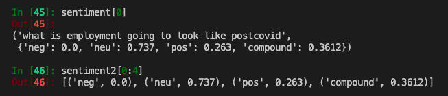
After we have appended each sentence (sentiment) and their polarity scores (sentiment2, negative, neutral, positive), we'll create data frames to store these values.
Then, we'll write the data frames to CSV to transition to R. Note that we set index to false when saving for CSV. Python starts counting at 0, while R starts at 1, so we're better off re-creating the index as a separate column in R.
NOTE: There are more efficient ways for what I'm doing here. My solution is to save two CSV files and move the work flow over to R for further data manipulation and visualization. This is primarily a personal preference for handling data frames and visualizations in R, but I should point out this can be done with pandas and matplotlib.
# nltk.download('vader_lexicon')

sid = SentimentIntensityAnalyzer()

sentiment = []
sentiment2 = []

for sent in sents:
    sent1 = sent
    sent_scores = sid.polarity_scores(sent1)
    for x, y in sent_scores.items():
        sentiment2.append((x, y))
    sentiment.append((sent1, sent_scores))
    # print(sentiment)

# sentiment
cols = ['sentence', 'numbers']
result = pd.DataFrame(sentiment, columns=cols)
print("First five rows of results: ", result.head())

# sentiment2
cols2 = ['label', 'values']
result2 = pd.DataFrame(sentiment2, columns=cols2)
print("First five rows of results2: ", result2.head())

# save to CSV
result.to_csv('sent_sentiment.csv', index=False)
result2.to_csv('sent_sentiment_2.csv', index=False)
Data Transformation
From this point forward, we'll be using R and the tidyverse for data manipulation and visualization. RStudio is the IDE of choice here. We'll create an R Script to store all our data transformation and visualization process. We should be in the same directory in which the above CSV files were created with pandas.
We'll load the two CSV files we saved and the tidyverse library:
library(tidyverse)

# load data
df <- read_csv("sent_sentiment.csv")
df2 <- read_csv('sent_sentiment_2.csv')
We'll create another column that matches the index for the first data frame (sent_sentiment.csv). I save it as df1, but you could overwrite the original df if you wanted.
# create a unique identifier for each sentence
df1 <- df %>%
    mutate(row = row_number())
Then, for the second data frame (sent_sentiment_2.csv), we'll create another column matching the index, but also use pivot_wider from the tidyr package. NOTE: You'll want to group_by label first, then use mutate to create a unique identifier.
We'll then use pivot_wider to ensure that all polarity values (negative, neutral, positive) have their own columns.
By creating a unique identifier using mutate and row_number(), we'll be able to join (left_join) by row.
Finally, I save the operation to df3 which allows me to work off a fresh new data frame for visualization.
# long-to-wide for df2
# note: first, group by label; then, create a unique identifier for each label then use pivot_wider

df3 <- df2 %>%
    group_by(label) %>%
    mutate(row = row_number()) %>%
    pivot_wider(names_from = label, values_from = values) %>%
    left_join(df1, by = 'row') %>%
    select(row, sentence, neg:compound, numbers)
Visualization
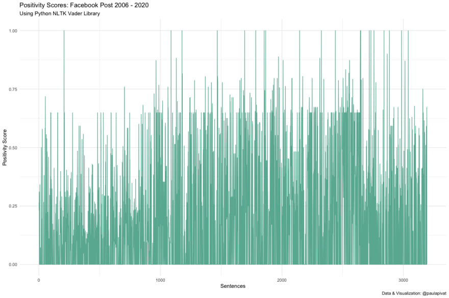
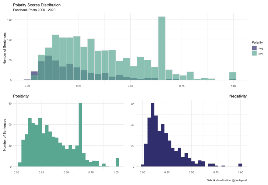
First, we'll visualize the positive and negative polarity scores separately, across all 3194 sentences (your numbers will vary).
Here are positivity scores:
Here are negativity scores:
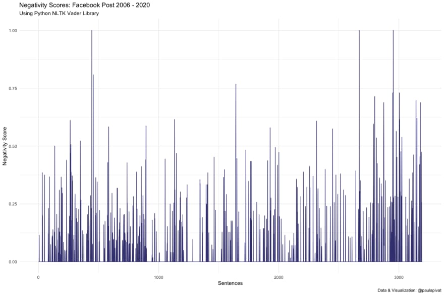
When I sum positivity and negativity scores to get a ratio, it's approximately 568:97 or 5.8x more positive than negative according to the Vader (Valance Aware Dictionary and Sentiment Reasoner).
The Vader module will take in every sentence and assign a valence score from -1 (most negative) to 1 (most positive). We can classify sentences as pos (positive), neu (neutral) and neg(negative) or as a composite (compound) score (i.e., normalized, weighted composite score). For more details, see vader-sentiment documentation.
Here is a chart to see both positive and negative scores together (positive = blue, negative = red, neutral = black).

Finally, we can also use histograms to see the distribution of negative and positive sentiment among the sentences:
Non-Normalized Data
It turns out the Vader module is fully capable of analyzing sentences with punctuation, word-shape (capitalization for emphasis), slang and even utf-8 encoded emojis.
So to see if there would be any difference if we implemented sentiment analysis without normalization, I re-ran all the analyses above.
Here are the two version of data for comparison. Top for normalization and bottom for non-normalized.
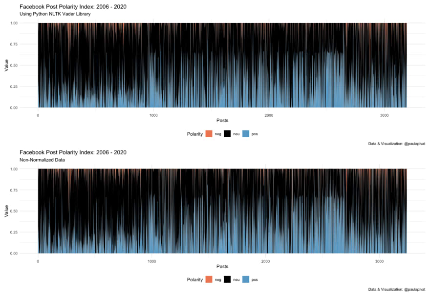
While there are expected slight differences, they are only slight.
Summary
I downloaded 14 years worth of Facebook posts to run a rule-based sentiment analysis and visualize the results, using a combination of Python and R.
I enjoyed using both for this project and sought to play to their strengths. I found parsing JSON straight-forward with Python, but once we transition to data frames, I was itching to get back to R.
Because we lacked labeled data, using a rule-based/lexicon-approach to sentiment analysis made sense. Now that we have a label for valence scores, it may be possible to take a machine learning approach to predict the valence of future posts.
References
- Hutto, C.J. & Gilbert, E.E. (2014). VADER: A Parsimonious Rule-based Model for Sentiment Analysis of Social Media Text. Eighth International Conference on Weblogs and Social Media (ICWSM-14). Ann Arbor, MI, June 2014.
For more content on data science, machine learning, R, Python, SQL and more, find me on Twitter.

Top comments (0)