Here we are going to build a classification model for theMushroom Classification Dataset. The model is going to classify if the mushroom is edible (e) or poisonous (p). Other attributes are:
You can find description of all the attributes following the kaggle link.
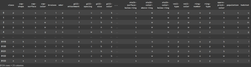
First let's import pandas and use it to read the downloaded dataset. Then we will display the downloaded dataset
m_df = pd.read_csv("/content/mushrooms.csv")
m_df
Output:
Now we should explore the dataset:
Check for unfilled column values:
m_df.isnull().sum()
Output:
class                       0
cap-shape                   0
cap-surface                 0
cap-color                   0
bruises                     0
odor                        0
gill-attachment             0
gill-spacing                0
gill-size                   0
gill-color                  0
stalk-shape                 0
stalk-root                  0
stalk-surface-above-ring    0
stalk-surface-below-ring    0
stalk-color-above-ring      0
stalk-color-below-ring      0
veil-type                   0
veil-color                  0
ring-number                 0
ring-type                   0
spore-print-color           0
population                  0
habitat                     0
dtype: int64
No columns have a missing value.
Now check for the datatypes of the dataset:
m_df.dtypes
Output:
class                       object
cap-shape                   object
cap-surface                 object
cap-color                   object
bruises                     object
odor                        object
gill-attachment             object
gill-spacing                object
gill-size                   object
gill-color                  object
stalk-shape                 object
stalk-root                  object
stalk-surface-above-ring    object
stalk-surface-below-ring    object
stalk-color-above-ring      object
stalk-color-below-ring      object
veil-type                   object
veil-color                  object
ring-number                 object
ring-type                   object
spore-print-color           object
population                  object
habitat                     object
dtype: object
As we can see there are no numerical columns.
After analyzing the dataset we should split it into two: the labels dataset and the features dataset.
X = m_df.drop("class", axis=1)
y = m_df["class"]
We can not train the model and test the predicted results on the same dataset, just as a student should not be writing an exam he was allowed to see in advance, so we have to split the dataset into testing and training:
from sklearn.model_selection import train_test_split

# The labels should be numerical so we replace all of the labels
# with ones and zeros
y.replace("p", 0, inplace=True)
y.replace("e", 1, inplace=True)
X_train, X_test, y_train, y_test = train_test_split(X,y,test_size=(0.2))
All the values in the dataset are in categorical form. The model can not learn anything from data in such form so we should onehot encode it - put in through a process of converting each categorical value into a new categorical column and assigning a binary value of 1 or 0 to those column. Also we might want to plot all of the mushroom samples so that we can better visualize the correlation of attributes to the labels. We can do that via dimension reduction, in this example - using PCA.
from sklearn.model_selection import train_test_split
from sklearn.preprocessing import OneHotEncoder
from sklearn.compose import ColumnTransformer

cat_features = [*X.columns]
cat_transformer = Pipeline(steps=[("onehot", OneHotEncoder(sparse=False)), ("pca", PCA(n_components=2))])

ct = ColumnTransformer(transformers=[("categories", cat_transformer, cat_features)])
ct.fit(X)
X_train_t = ct.transform(X_train)
X_test_t = ct.transform(X_test)
Plotting the PCA graph:
plt.scatter(X_train_t[:, 0], X_train_t[:, 1], alpha=0.4, color="lightblue");

We can also see correlations of different features to the labels on the heatmap:
sns.heatmap(pd.get_dummies(m_df).corr())

Now we can finally start training our model. We only have to distinct labels, so we should be using the sigmoid activation function, as it is going to be returning us values of the range from 0 to 1, as well as using binary_crossentropy. We are also going to use the LearningRateSchedulercallback to try and find the ideal learning rate by analyzing loss and accuracy at different learning rates from (1e-4 * (10**(1/15))) (0.000116591440118) to (1e-4 * (10**(100/15))) (464.158883361)
model = tf.keras.Sequential([
    tf.keras.layers.Dense(10, activation="relu"),
    tf.keras.layers.Dense(30, activation="relu"),
    tf.keras.layers.Dense(1, activation="sigmoid")
])

model.compile(loss="binary_crossentropy", optimizer=tf.keras.optimizers.Adam(), metrics=[tf.keras.metrics.binary_crossentropy, "accuracy"])

lr_cb = tf.keras.callbacks.LearningRateScheduler(lambda epoch: 1e-4 * (10**(epoch/15)))

history = model.fit(X_train_t, y_train, epochs=70, verbose=1,  callbacks=[lr_cb])
We can visualize the history of the training process of our model:
hist = pd.DataFrame(history.history).drop("binary_crossentropy", axis=1)
hist.plot()

As we can see on the graph the accuracy of the model starts dropping when the learning rate increases beyond a certain point.
Let's look at the correlation of the learning rate and the loss curve closer:
lrs = 1e-4 * (10**(np.arange(0,70)/15)) # generate an array of
# learning rates with the same number of epochs
plt.semilogx(lrs, hist.loss)

The loss is steeply decreasing from 10e-4 to 10e-3. We should take te value closer to the lowest point of the curve (10e-3), the value is going to be equal to around 0.0097 (Which is almost the exact same as the Adam's default learning rate).
Now let's fit the model with the ideal learning rate:
model = tf.keras.Sequential([
    tf.keras.layers.Dense(10, activation="relu"),
    tf.keras.layers.Dense(30, activation="relu"),
    tf.keras.layers.Dense(1, activation="sigmoid")
])

model.compile(loss="binary_crossentropy", optimizer=tf.keras.optimizers.Adam(learning_rate=0.0097), metrics=[tf.keras.metrics.binary_crossentropy, "accuracy"])

history = model.fit(X_train_t, y_train, epochs=15, verbose=1)
Now we can use the testing dataset to make predictions with our model and draw a confusion matrix to better visualize the results:
y_pred = np.round(model.predict(X_test_t)[:, 0])
ConfusionMatrixDisplay.from_predictions(y_true=y_test, y_pred=y_pred);

Now lets write a function that is going to return different metrics based on the model's predicitons and the actual values and use it to evaluate our model:
def metrics(y_test, y_pred):
    f1 = f1_score(y_test, y_pred)
    rec = recall_score(y_test, y_pred)
    acc = accuracy_score(y_test,y_pred)
    prec = precision_score(y_test,y_pred)
    return f"Accuracy: {round(acc, 2)}, Precision: {round(prec, 2)}, Recall: {round(rec, 2)}, F1: {round(f1, 2)}"
metrics(y_test, y_pred)
Output:
Accuracy: 0.94, Precision: 0.96, Recall: 0.93, F1: 0.94
Now our model is finished! Hope this article was helpful and thank you for a read!

Top comments (1)
Neural networks for mushroom classification are fascinating, but relying solely on AI for edibility checks can be risky. While models can achieve high accuracy, they aren’t foolproof—misclassification could have serious consequences. That’s why expert knowledge and proper identification techniques remain crucial. For those interested in learning more about safe foraging and distinguishing edible mushrooms, fungiape.com does a great job of explaining key identification factors. Combining AI predictions with real-world expertise seems like the best approach. Have you tested any models yourself, or do you prefer traditional field guides for identification?