
Introduction
Compared with V1.0, NebulaGraph, a distributed graph database, has been significantly changed in V2.0. One of the most obvious changes is that in NebulaGraph 1.0, the code of the Query, Storage, and Meta modules are placed in one repository, while from NebulaGraph 2.0 onwards, these modules are placed in three repositories:
- nebula-graph: Mainly contains the code of the Query module.
- nebula-common: Mainly contains expression definitions, function definitions, and some public interfaces.
- nebula-storage: Mainly contains the code of the Storage and Meta modules.
This article introduces the overall structure of the Query layer and uses an nGQL statement to describe how it is processed in the four main modules of the Query layer.
Architecture
This figure shows the architecture of the Query layer. It has four submodules:
- Parser: Performs lexical analysis and syntax analysis.
- Validator: Validates the statements.
- Planner: Generates and optimizes the execution plans.
- Executor: Executes the operators.

3. Source Code Hierarchy
Now, let’s look at the source code hierarchy under the nebula-graph repository.
|--src
|--context // contexts for validation and execution
|--daemons
|--executor // execution operators
|--mock
|--optimizer // optimization rules
|--parser // lexical analysis and syntax analysis
|--planner // structure of the execution plans
|--scheduler // scheduler
|--service
|--util // basic components
|--validator // validation of the statements
|--visitor
4. How a Query is Executed
Starting from the release of NebulaGraph 2.0-alpha, nGQL gets to support vertex IDs of the String type. It is working to support vertex IDs of the Int type in NebulaGraph 2.0 to get compatible with NebulaGraph 1.0.
To introduce how the Query layer works, let’s take an nGQL statement like GO FROM "Tim" OVER like WHERE like.likeness > 8.0 YIELD like._dst as an example. Its data flow through the Query layer is shown in the following figure.

When the statement is input, it is processed as follows.
Stage 1: Generating an AST
In the first stage, the statement is parsed by the Parser (composed of Flex and Bison) and its corresponding AST is generated. The structure of the AST is shown in the following figure.
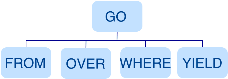
In this stage, the Parser intercepts the statements that do not conform to the syntax rules. For example, a statement like GO "Tim" FROM OVER like YIELD like._dst will be directly intercepted in this stage because of its invalid syntax.
Stage 2: Validation
In the second stage, the Validator performs a series of validations on the AST. It mainly works on these tasks:
When parsing the OVER , WHERE , and YIELD clauses, the Validator looks up the Schema and verifies whether the edge and tag data exist or not. For an INSERT statement, the Validator verifies whether the types of the inserted data are the same as the ones defined in the Schema.
For multiple statements, like $var = GO FROM "Tim" OVER like YIELD like._dst AS ID; GO FROM $var.ID OVER serve YIELD serve._dst, the Validator verifies $var.ID: first to see if var was defined, and then to check if the ID property is attached to the var variable. If $var.ID is replaced with $var1.ID or $var.IID , the validation fails.
The Validator infers what type the result of an expression is and verifies the type against the specified clause. For example, the WHERE clause requires the result to be a Boolean value, a NULL value, or empty.
Take a statement like GO FROM "Tim" OVER * YIELD like._dst, like.likeness, serve._dst as an example. When verifying the OVER clause, the Validator needs to query the Schema and replace * with all the edges defined in the Schema. For example, if only like and serve edges are defined, the statement is as follows.
GO FROM "Tim" OVER serve, like YIELD like._dst, like.likeness, serve._dst
For an nGQL statement with the PIPE operator, such as GO FROM "Tim" OVER like YIELD like._dst AS ID | GO FROM $-.ID OVER serve YIELD serve._dst, the Validator verifies $-.ID . In the example statement, the ID property in the second clause was already defined in the previous clause, so the second clause is verified legal. If $-.ID is changed to $-.a , where a was not defined, the second clause is illegal.
Stage 3: Generating an Execution Plan
When the validation succeeds, an execution plan is generated in Stage 3. Its data structure is stored in the src/planner directory, with the following logical structure.

Query Execution Flow
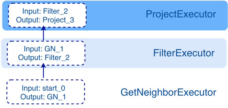
The generated execution plan is a directed acyclic graph where the dependencies between nodes are determined in the toPlan() function of each module in the Validator. As shown in the preceding figure, the Project node depends on the Filter node, the Filter node depends on the GetNeighbor node, and so on, up to the Start node.
During the execution stage, the Executor generates an operator for each node and starts scheduling from the root node (e.g., the Project node in this example). If the root node is found to be dependent on other nodes, the Executor recursively calls the nodes that the root node depends on until it finds a node that is not dependent on any node (e.g., the Start node in this example), and then starts execution. After the execution, the Executor continues executing the node that depends on the executed node (e.g., the GetNeighbor node in this example), and so on, until the root node is reached.
Query Data Flow
The input and output of each node are also determined in toPlan(). Although the execution is performed in the order defined in the execution plan, the input of each node can be customized and does not completely depend on the previous node, because the input and output of all nodes are actually stored in a hash table, where the keys are the names customized during the creation of each node. For example, if the hash table is named as ResultMap, when creating the Filter node, you can determine that the node takes data from ResultMap["GN1"], then puts the result into ResultMap["Filter2"], and so on. All these work as the input and output of each node. The hash table is defined in src/context/ExecutionContext.cpp under the nebula-graph repository. The execution plan is not really executed, so the value of each key in the associated hash table is empty (except for the starting node, where the input variables hold the starting data), and they will be computed and filled in the Executor stage.
This is a simple example. A more complex one will be shown at the end for you to better understand how an execution plan works.
Stage 4: Optimizing the Execution Plan
An execution plan generated in the preceding stage can be optimized optionally. In the etc/nebula-graphd.conf file, when enable_optimizer is set to true, the execution plans will be optimized. In this example, when optimization is enabled, the data flow is as follows.

As shown in the preceding figure, the Filter node is integrated into the GetNeighbor node. Therefore, when the GetNeighbor operator calls interfaces of the Storage layer to get the neighboring edges of a vertex during the execution stage, the Storage layer will directly filter out the unqualified edges internally. Such optimization greatly reduces the amount of data transfer, which is commonly known as filter push down.
In the execution plan, each node directly depends on other nodes. To explore equivalent transformations and to reuse the same parts of an execution plan, such a direct dependency between nodes is converted into an OptGroupNode to OptGroup dependency. Each OptGroup contains an equivalent set of OptGroupNodes, and each OptGroupNode contains one node in the execution plan. An OptGroupNode depends on an OptGroup but not on other OptGroupNodes. Therefore, from one OptGroupNode, many equivalent execution plans can be explored because the OptGroup it depends on contains different OptGroupNodes, which saves storage space.
All the optimization rules we have implemented so far are considered as RBO (Rule-Based Optimization), which means the plans optimized based on the rules must be better than their original versions. The CBO (Cost-Based Optimization) feature is under development. The optimization process is a “bottom-up” exploration process: For each rule, the root node of the execution plan (in this case, the Project node) is the entry point, along the node dependencies, the bottom node is found, and then from the bottom node, the OptGroupNode in each OptGroup is explored to see if it matches the rule, until the entire execution plan can no longer apply the rule. Then, the next rule is explored.
This figure shows the optimization process of this example.

As shown in the preceding figure, when the Filter node is explored, it is found that its children node is GetNeighbors, which matches successfully with the pre-defined pattern in the rule, so a transformation is initiated to integrate the Filter node into the GetNeighbors node, the Filter node is removed, and then the process continues to the next rule.
The optimized code is in the src/optimizer/ directory under the nebula-graph repository.
Stage 5: Execution
In the fifth stage, the Scheduler generates the corresponding execution operators against the execution plan, starting from the leaf nodes and ending at the root node. The structure is as follows.
Each node of the execution plan has one execution operator node, whose input and output have been determined in the execution plan. Each operator only needs to get the values for the input variables, compute them, and finally put the results into the corresponding output variables. Therefore, it is only necessary to execute step by step from the starting node, and the result of the last operator is returned to the user as the final result.
An Example Query
Now we will get acquainted with the structure of an execution plan by executing a FIND SHORTEST PATH statement.
Open nebula-console and enter the following statement.
FIND SHORTEST PATH FROM "YAO MING" TO "Tim Duncan" OVER like, serve UPTO 5 STEPS
To get the details of the execution plan of this statement, precede it with the EXPLAIN.
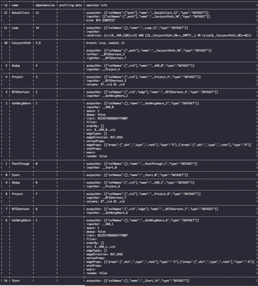
The preceding figure shows, from left to right, the unique ID of each node in the execution plan, their names, the IDs of their dependent nodes, the profiling data (information about the execution of the PROFILE command), and the details of each node (including the names of the input and output variables, the column names of the output results, and the parameters of the node).
To visualize the information, you can follow these steps:
- Use EXPLAIN format="dot" instead of EXPLAIN. nebula-console can generate the data in the DOT format.
- Open the Graphviz Online website and paste the generated DOT data. You can see the structure as shown in the following figure. This structure corresponds to the execution flow of the operators in the execution stage.

The shortest path algorithm uses the two-way breadth-first search algorithm, expanding from both “YAO MING” and “Tim Duncan”, so GetNeighbors, BFSShortest, Project, and Dedup have two operators, respectively, the input is connected by the PassThrough operator, and the path is stitched by the ConjunctPath operator. The LOOP operator then controls the number of steps to be extended outward, and it can be seen that the input of the DataCollect operator is actually taken from the output variable of the ConjunctPath operator.
The information of each operator is in the src/executor directory under the nebula-graph directory. Feel free to share your ideas with us on GitHub: https://github.com/vesoft-inc/nebula or the official forum: https://discuss.nebula-graph.io/
Originally published at https://nebula-graph.io on March 16, 2021.

Top comments (0)