
Introduction
As a Performance Engineer, I have observed multiple cases where my intuition has failed me while trying to make inferences about data. Since it is imperative to get good at making decisions with data, emboldening your "BS" detection skillset is of paramount importance for any engineer.
This blog post is the first of 3 that goes over some ways you or others can lie with data from performance analysis such as Benchmarks or Regression detection based tooling.
How To Lie With Small Number of Data Points
A data set with a small number of data points isn't sufficient enough to represent a true distribution especially if the data is littered with anomalous values.
Visual Perspective: Histogram
Consider the two data points both generated from a Standard Normal Distribution (As an aside, I have never observed any real performance data that follows a normal distribution but for the sake of exposition, I'll stick with this example):
For a sample size of n = 10
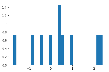
Visually, the histogram has no semblance of the standard normal distribution or even a normal distribution.
For a sample size of n = 10,000
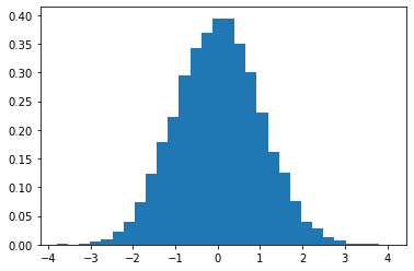
This distribution is more like the standard normal distribution, the real population from which we sample from indicating that the more the samples, the better we are off in terms of making decisions.
The code that generated these is the following:
Statistical Perspective: Standard Error, Margin of Error and Confidence Intervals
Standard Error
The Standard Error gives us a measure of accuracy of how close the sample is to the true mean. The higher the standard error the less accurate we are in terms of guessing the true mean of a population.
The formula for standard error is:
| Variable | Description |
|---|---|
| se | Standard Error |
| s | Standard Deviation of the Sample |
| n | Number of Samples |
From the formula, we notice that a lower 'n' under the condition of a lower number of samples, we are less accurate in guessing the true statistic such as the mean of a population as the Standard Error is higher.
Margin of Error
The Margin of Error is the Standard Error multiplied by a critical value:
Formulaically, the margin of error is given by:
Confidence Intervals
Confidence Intervals are ranges between which the population statistic can be in with the margin of error as the "radius" or allowable leverage of error. For example, a confidence interval of 99% indicates that 99% of all confidence intervals with confidence level = 99% include the true population statistic.
For example, for the mean of a population based on a sample is given by:
Since the confidence interval does inherently rely on the number of samples, the conjecture that the "higher number of samples will give us a higher level of confidence about the said population statistic" is valid.
Conclusion
Here are the lessons I have learnt over the years regarding the number of samples:
- Be sure to ask the number of data points the descriptive statistics were based off of. If the number of samples are low, inaccurate inferences from the data are possible.
- Make sure that even with seemingly high number of samples, the data is littered with anomalies; find out how to decrease these.
- Sometimes it's infeasible to get more samples - for these cases, make sure your anomalous values are as low as possible.
- Most importantly: always question the data.

Top comments (0)