
When working with datasets and using machine learning processes, it’s usual to normalize our data before using it. Whenever we’re using any machine learning algorithm that involves euclidean distance, data should be scaled. Whenever using KNN, Clustering, linear regression, all deep learning and artificial network algorithms, data should be scaled. There are though, many ways that this can be done. So what scaling method should you use?
In this post I’ll explain why it is an important thing to do, and go through Scikit Learn different scaling models and talk about their differences.
Normalization and Standardization
Both of these are common techniques used when preparing data before undergoing any machine learning procedures. They aim to change the values of numeric columns in a dataset, to have them all be in a common scale, without distorting their range of values or losing information. For instance, if one of your columns have values that range from 0 to 1, while another ranges from 10,000 to 100,000, that difference may cause problems when combining those values when modelling the data.
The big difference between them is that Normalization usually means rescaling values into a range between 0 and 1, while Standardization usually means rescaling the data to have a mean of 0, and a standard deviation of 1 (in other words, replaces point values with their z-score).
Standardization
Here’s the mathematical formula for standardization:

The mean here is the mean of the feature values, sd is the standard deviation of the feature values. In standardization, your values are not restricted to a particular range.
Normalization
This can take a few different forms. One of the most common ones is called the Min-Max scaling. Here’s the formula for MinMax:
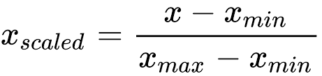
X-max and X-min are, respectively, the maximum and minimum values of the feature.
You can see that, if X is equal to X-min, X’ value will be 0, while if X is equal to X-max, X’ value will be 1. Every other number will fall between the two.
Shaping Data with Python
I’ll use a couple of models here to give you a better understanding of what these methods are doing.
First, I’ll use distance from London to create a quick model to compare house prices. Here’s the information:
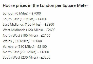
Now let’s get them in numpy array form, and shape them as columns, so we can transform them later on:
Import numpy as np
X_property_dist = np.array([0, 10, 105, 120, 180, 200, 210, 220, 230]).reshape(-1, 1)
y_price = np.array([6000, 4100, 2200, 2600, 2100, 2000, 2100, 1800, 2200]).reshape(-1, 1)
Now we’ll take a look of how this data look like:
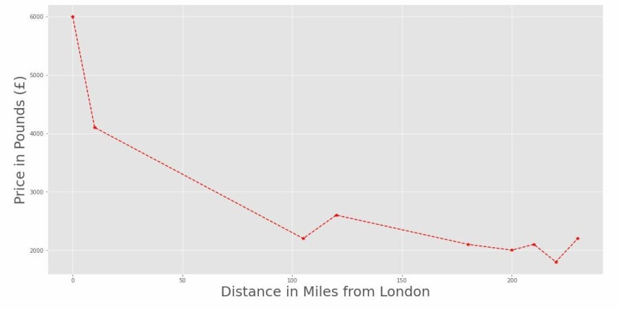
As you can see, the scales here range from 0 to 230 in the x-axis, while they vary from 1800 to 6000 in the y-axis. Our task is to transform this data so they’re all in the same scale. With Sklearn you can easily do that with some preprocessing methods. We’ll start with the Standard Scaler, that Standardizes the data:
from sklearn.preprocessing import StandardScaler

ss_scaler = StandardScaler() # Instantiate the scaler

X_dist_scl_ss = ss_scaler.fit_transform(X_property_dist)
y_price_scl_ss = ss_scaler.fit_transform(y_price)
These methods will transform the data we previously had by getting their mean to 0 and make their standard deviation be 1. Here are the results:
X_dist_scl_ss:

y_price_scl_ss:
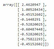

The data now has a very different scale, and now is easier to compare unit changes between the two axis. Important to note though, that there was no distortion in any values, which means the graph we’re seeing looks exactly the same as the previous one, bearing the scale.
To further exemplify this, this set of graphs shows the effects of a Standard Scaler in 3 normally distributed arrays:
np.random.seed(2022)
df = pd.DataFrame({
    'x1': np.random.normal(0, 2, 10000),
    'x2': np.random.normal(5, 3, 10000),
    'x3': np.random.normal(-5, 5, 10000)
})

scaler = StandardScaler()
scaled_df = scaler.fit_transform(df)
scaled_df = pd.DataFrame(scaled_df, columns=['x1', 'x2', 'x3'])

fig, (ax1, ax2) = plt.subplots(ncols=2, figsize=(12, 10))

ax1.set_title('Before Scaling')
for i in range(1, 4):
    sns.kdeplot(df[f'x{i}'], ax=ax1)
ax2.set_title('After Standard Scaler')
for i in range(1, 4):
    sns.kdeplot(scaled_df[f'x{i}'], ax=ax2)
plt.show()
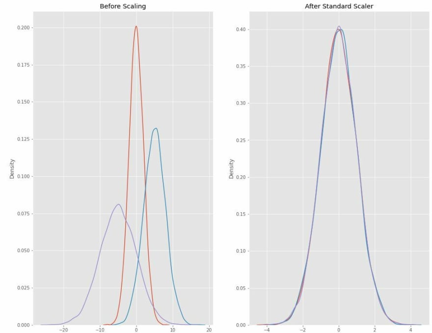
So here you can clearly see how all their means were shifted to 0, and the standard deviation was now set to 1.
Now we’ll take a look at what MinMax, one of the most commons normalizers, does to these two sets of data:
from sklearn.preprocessing import MinMaxScaler

mm_scaler = MinMaxScaler() # Instantiate the scaler

y_price_mm = mm_scaler.fit_transform(y_price)
X_dist_mm = mm_scaler.fit_transform(X_property_dist)
These methods will scale the data down so that the minimum value is 0, and the maximum is 1. Let’s take a look at the results:
X_dist_scl_mm:

y_price_scl_mm:

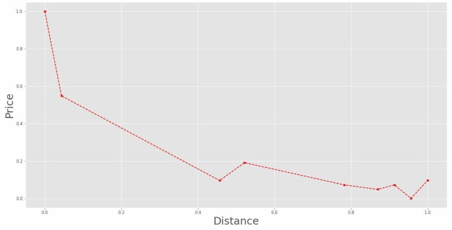
This makes it even easier to compare the two. All values are now in a scale between 0 and 1, and since, again, there was no distortion in the values, the last graph looks the same as both previous ones.
Let’s take a quick look at the effect the MinMax scaler had in our previous example as well:

Now the means of the curves are not exactly the same, but you can see that all the x-axis values fall within 0 and 1.
Other Scalers
Scikit Learn provides a good number of different scalers whose usefulness depend heavily on the type of data we're looking at, mostly looking at how it is distributed and if it contains outliers. Let's go through a few of them:
Robust Scaler: This scaler scales the data around the median according to the quantile range. This comes in handy when your data has outliers that influence the mean too much, making them interfere less with the results. Any method that is strong to outliers is considered to be Robust.
Max Absolute Scaler: Instead of fitting the data within a 0 to 1 range like the MinMax, the MaXAbs scaler sets the maximum value to be 1, but doesn't define a minimum. The data here is not shifted or centred around any point, maintaining sparsity.
Power Transformer: Makes the data more Gaussian-like. It's useful for situations where approximation to normality is needed.
Normalizer: Each sample is rescaled according to norm, either L1, L2 or max. This is applied row-wise, so each rescaling is independent from the others. Here, max does to a row what MaxAbsScaler does for features, l1 uses the sum of all values as norm, giving equal penalty to parameters, and l2 uses the square root of the sum of all squared values, increasing smoothness.
All other preprocessing and normalization methods from Scikit Learn can be found here.
How to choose?
Usually when you get to a conclusion stage of a post like this, you find clear and defined rules to what to do in different situations. Unfortunately, that is not the case here. There isn’t a simple way to be 100% sure on what scaling technique to use all of the time. Sometimes one can yield better results, but depending on the data, another one might be more appropriate. Above I described a little how to chose from a few of these methods. Below is a quick overview comparing just the main topic of this post:
- Standardization does not affect outliers, since it doesn’t have a bounding range. It is useful though if your data follows a Gaussian Distribution (also called Normal Distribution).
- Normalization is less useful if your data already follows a Normal Distribution. It's necessary when using a prediction algorithm based on weighted relationships between data points.
Predictive modeling problems can be complex, and knowing how to best scale your data may not be simple. There is no knowing the best technique for every scenario. Sometimes even multiple transformations are ideal. What we should aim to then is to create different models, that shape the data in different ways, run our models and analyse their outcomes.
References:
- Preprocessing with Sklearn
- Compare Scalers on data with Outliers
- StandardScaler and MinMaxScaler in Python
- Rescaling Data for Machine Learning in Python with Scikit-Learn
- Feature Scaling with Scikit-Learn
- How, When, and Why Should You Normalize / Standardize / Rescale Your Data?
- Understanding the Difference Between Normalization vs. Standardization
- Standardization Vs Normalization- Feature Scaling

Top comments (0)