In this blog I am going to compare two approaches to image classification: support vector machine (a classical machine learning method) vs multilayer perceptron (neural network).
Now, I am not going to use a convolutional neural network as that wouldn't be a fair fight given that CNNs automatically learn hierarchical features from raw pixel data, eliminating the need for explicit feature engineering. Rather, I am going to manually extract important features when needed and run the resulting dataset through both methods.
Metrics
Given that we are dealing with classification, the metrics predominantly used to compare model performance are recall, precision and accuracy.
Recall measures the model's ability to correctly identify all relevant instances, specifically the ratio of correctly predicted positive observations to the total actual positives. It is calculated as True Positives / (True Positives + False Negatives).
Precision measures the accuracy of positive predictions made by the model, specifically the ratio of correctly predicted positive observations to the total predicted positives. It is calculated as True Positives / (True Positives + False Positives).
Accuracy measures the overall correctness of the model's predictions across all classes. It is calculated as (True Positives + True Negatives) / Total Observations.
Taking into account that all 3 of our datasets are balanced, meaning that every class is evenly represented in terms of observations, accuracy will be our main metric for comparing model performance.
Models
Support Vector Machines (SVM) constitute a powerful class of supervised learning models proficient at classification and regression tasks. The fundamental principle of SVM involves identifying an optimal hyperplane that separates classes in the input space. In the case of linear SVM, this entails finding a hyperplane that maximizes the distance between the hyperplane and the nearest data points from different classes. Lineal SVM is highly effective for linearly separable datasets, providing robustness against overfitting and demonstrating efficiency in high-dimensional spaces without requiring complex computations.
 [image 1]
The Radial Basis Function SVM (RBF), extends the capability of SVM to handle non-linearly separable data. By employing a kernel trick, it transforms the data into a higher-dimensional space, enabling the creation of non-linear decision boundaries. Consider the figure below, at first you can’t draw a line that accurately separates the 2 classes, but if you transform those points intoa higher dimension you can find a plane that achieves 100% separation. This flexibility in modeling intricate relationships makes RBF SVM suitable for diverse datasets with non-linear patterns.
 [image 2]
Multilayer Perceptron (MLP) represents a class of artificial neural networks structured with multiple layers, including an input layer, one or more hidden layers, and an output layer. MLPs leverage non-linear activation functions (such as ReLU) within each neuron, allowing them to learn complex (often non linear) relationships between inputs and outputs. Through forward propagation, data is processed through the network, and by utilizing backpropagation (a technique involving gradient descent) the weights are iteratively adjusted to minimize prediction errors. MLPs excel in feature learning, automatically extracting and representing essential features from raw data and reducing the need for explicit feature engineering. However, the use of feature extraction is still needed in cases such as this one, where HD images result in a large enough number of features that the computational effort becomes too costly to be a practical approach.
 [image 3]
Datasets
Before jumping into our results, I want to go over the datasets we're using.
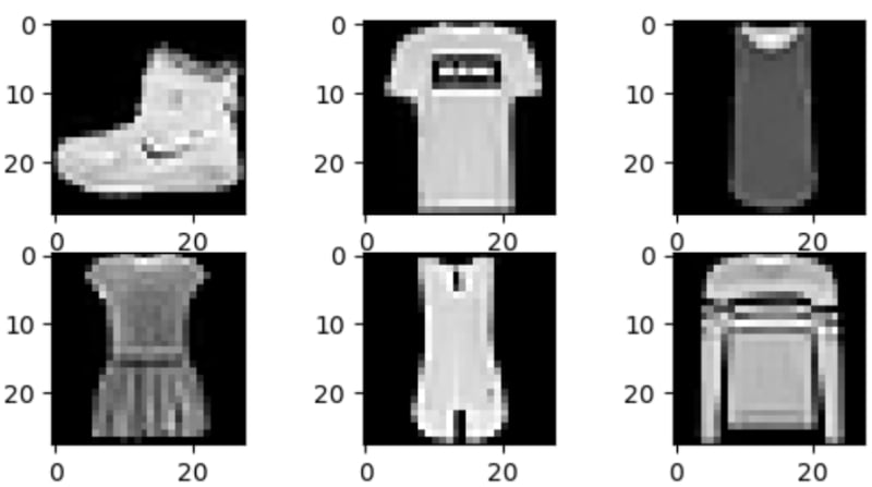
First off we have the Fashion-MNIST Dataset, it's comprised of 70,000 grayscale images, meticulously scaled and normalized. It includes 60,000 images for training and 10,000 for testing, each depicting various fashion items categorized into 10 classes. These images, sized at 28x28 pixels, offer a diverse collection of wearable items, making it a valuable resource for machine learning tasks like image classification and pattern recognition. The dataset's size and organization make cross validation unnecessary, simplifying training.
The classes present are the following:
- T-shirt
- Trouser
- Pullover
- Dress
- Coat
- Sandal
- Shirt
- Sneaker
- Bag
- Ankle Boot
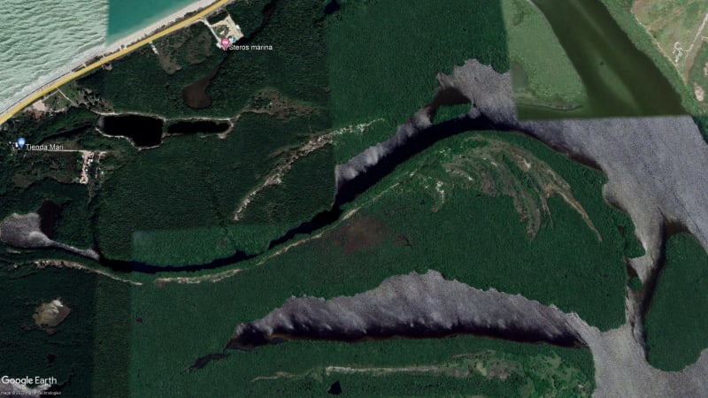
The second dataset has approximately 2,000 high-definition images of different landscapes across Mexico obtained from satellite captures. Each image showcases distinct environmental settings categorized into six classes: Water, Forest, City, Agriculture, Desert, and Mountain. Given that these are HD colored images we need to perform feature extraction in order to train our models. First we resized each image to 128x128 pixels, then we computed the color histograms (RGB) and concatenated them to represent the color distribution in the image. Then we captured texture features in the image by converting to grayscale and computing a Gray Level Co-occurrence Matrix (GLCM). These extracted features are concatenated into a single feature vector for each image along with its class (target variable).
The classes present are the following:
- Water
- Forest
- City
- Crops
- Desert
- Mountain
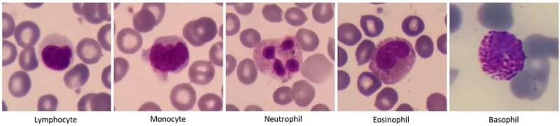
The third and final dataset is comprised of blood images using a microscope, taken by our team with the purpose of classifying the different type of white blood cells present. Given that these images share characteristics with the satellite dataset such as HD resolution and color, we also need to perform feature extraction. In the same way as the satellite dataset, we computed the color histograms and computing the GLCM to create our feature vectors for each image.
The classes present are the following:
- Neutrophils
- Monocytes
- Eosinophils
- Basophils
- Lymphocytes
- Erythroblasts
Methodology and Results
Now that we know how our chosen models work, we can start with the training phase. We are using scikit-learn to import both SVC (support vector classification) and MLPClassifier (multilayer perceptron classifier).
Using each dataset, I first trained the both linear and radial based SVM models using cross validation (except in the case of the fashion dataset due to the high number of observations) and evaluated them using accuracy.
We can then proceed to train our MLP neural networks using a parameter grid to find the best hiperparameters for each dataset, and in the case of the Satellite and Blood datasets we used 5 fold cross validation via scikit-learn's StratifiedKFold.
These were the results in terms of accuracy:

Fashion dataset
Lineal SVM: 85%
Radial Base SVM: 88%
MLP Neural Network: 90%
We can see that Radial Base SVM outperformed Lineal SVM which might indicate that the dataset benefited from projection into higher dimension in order to be sepparable. Alas, the Neural Network still outperformed both models.
Satellite dataset
Lineal SVM: 82%
Radial Base SVM: 79%
MLP Neural Network: 86%
Both SVM models achieved a similar accuracy score, but the Neural Network substantially outperformed the other models.
Blood dataset
Lineal SVM: 95%
Radial Base SVM: 96%
MLP Neural Network: 96%
Here we can see that all models had similar performance with a high accuracy score of 95-96%.
Here the Neural Network was the high performer! Across the Fashion-MNIST dataset, the Radial Basis SVM achieved an 88% accuracy, while the MLP soared ahead with 90%. Similarly, in the satellite dataset, SVMs reached 79% to 82% accuracy, but the MLP secured an 86% accuracy score. Notably, in the blood cell images, both SVMs and the MLP achieved high accuracy, around 95% to 96%, indicating a balanced performance.
Conclusion
When comparing Support Vector Machines (SVM) and Multilayer Perceptron (MLP) for image classification across diverse datasets – Fashion-MNIST, satellite landscapes, and blood cell images – the MLP consistently outperformed SVMs in accuracy. This might be attributed to the MLP's inherent ability to automatically learn complex relationships within the data.
In contrast, SVMs, while powerful, often require extensive feature manipulation to achieve optimal results, particularly in datasets with intricate features and complex patterns such as the satellite image dataset.
The MLP's consistent superiority in accuracy signifies its adaptability and efficiency in image classification, allowing it to outperform other models and positioning it as a potent choice in this domain.
References
Gandhi, R. (2018, June 7). Support Vector Machine — Introduction to Machine Learning Algorithms. Medium; Towards Data Science. https://towardsdatascience.com/support-vector-machine-introduction-to-machine-learning-algorithms-934a444fca47Support
Vector Machine SVM Algorithm. (2021, January 20). GeeksforGeeks; GeeksforGeeks. https://www.geeksforgeeks.org/support-vector-machine-algorithm/
Images:

Top comments (0)