TLDR

While machines may have an easy time understanding numbers, it means nothing if there’s no meaning behind them. Learn techniques to scale to your numerical data, such as standardization and normalization to better grasp the correlation of your data.

Outline

• Recap
• Before we begin
• Numerical data types
• Why we scale
• Types of scaling
• Scaling with Pandas
• Use of numerical data

Recap

Last time, we looked at qualitative data, where we labeled the categories and assigned weights to data to make it machine readable. This time, we’re going to look at quantifiable data, aka numbers, and assign meanings to them through applying scales.

We’ll be looking at the different types of numerical data, discrete and continuous, as well as the algorithm or mathematical formula behind it. Finally, we’ll wrap it up by scaling all numerical values in our dataset.

Before we begin

This guide will use the big_data dataset, collected for a marketing campaign. It contains data on a customer’s personal life, to analyze and replicate their decision making. It is recommended to read the introductory guide first to understand how to calculate min, max, and standard deviation as we’ll be using it in our equations to scale the data.

Numerical data types

Quantitative data, also known as numerical data, is data that is represented by a numerical value. This can be discrete data, which represents a count of how many times something happened. On the other hand, there’s continuous data that stretches infinitely and is uncountable, such as time.

Discrete data

This type of data is fixed and each value in between can be represented as an equal amount of meaning. Due to this, examples of data that answers “how many” make great samples of discrete data. For a marketing campaign, this is usually how many times something is clicked, or how much something costs.

It’s easy to compare discrete data across two users. A user who clicks more on the webpage is likely to be more engaged than the other user that visits the website and doesn’t click on anything. There’s a bit more special math we can do to assign difference in meanings to discrete data, such as a user clicking on the purchase button versus a user clicking on the logout button, but we won’t go too into detail in this guide.

Continuous data

This data is contrary to discrete. Continuous data doesn’t answer the question of “how many”, because it’s a value that’s measured in a unit that is infinite. Most datasets that have continuous data would be a measure of time. Time is considered to be infinite because the meaning between finishing an hour due before, and hour after starting. For instance, I may want to reward someone for completing early, or take note of someone procrastinating until the last minute. In the end, the treatment or behavioral pattern the data reveals is different.

Why we scale

In order to fully grasp why knowing which type of numerical data matters, we must first understand how machines think. Machines are very literal, as we saw when working with categorical data, numbers will inherently carry a weight, and in practice these numbers can grow large and require a long time to do calculations or plot if left unchecked. This is where scaling comes in. Scaling reduces the values so that the data is easier to calculate, visualize, and remove bias.

Systematic bias

Systematic bias occurs when there is a large amount of data with respect to another part of the data. In this case, it can be an outlier, where the data contains areas with anomalies, a datapoint with a larger deviation compared to others. In this case, we can apply a technique called normalization which reduces the impact of outliers on our data.

Range of Data

In addition, scaling plays a big role in training time by shrinking the ranges. By reducing values that are extremely large into smaller values within a much smaller range, the calculations of each value is also decreased which helps with speed. A common example we’ll get into next is normalization, which shrinks all values into the range of [0,1], 0 to 1 inclusive.

Types of Scaling

Now that we understand the differences between the two types of numerical data and why we should scale, we may begin to identify a scaling approach that best fits each type of data. There are two scaling methods that we’ll go through, standardization, and normalization.

Normalization (Min-Max)

The 1st type of scaling we’ll go over is normalization, which compares the current value against the highest and lowest values and finds the average. Due to needing a max and a min value, Min-Max normalization is used for discrete sets of data which are countable and finite.

The pros of using Min-Max is that it’s faster to calculate, due to using simple mathematical operations, and easy to graphically view as the result is very linear.

On the downside, it has many restrictions when choosing to use it. In the case of continuous sets of data, you are unable to use normalization since the meaning behind the difference in values isn’t consistent. In addition, calculating normalization uses the minimum and maximum, so any outliers or abnormal minimums and maximums can greatly skew the output.

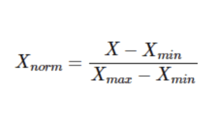Formula for Min-Max Normalization

Standardization (Z-Score)

Another type of scaling is through standardization. This is useful for continuous datasets that have no end in sight, but can also be used on discrete data. By standardizing the values you can assign meaning with respect to each other datapoint instead of a human assumption.

For this guide, we’ll be following the Z-score method of standardization, which takes the value and subtracts the mean to find the difference, then divides it by the standard deviation. When choosing standardization, it’s worth noting that since there’s no min or value, outliers won’t affect your data as much.

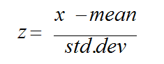Formula for Z-Score Standardization

Scaling with Pandas

Looking back at our dataset, we’ll begin to scale the numbers to assign meaning. Starting off by looking at the dataset, let’s break down the columns into only the relevant numerical data. Then break it down further into discrete data that can be normalized, and continuous data which cannot be normalized. Sklearn has functions that calculate standardization and min-max normalization, but for this guide we’ll be implementing it with the raw functions of Pandas to practice understanding and implementing the equation.

According to the output of df.info, we’ll want to keep any relevant values that are an int or float data type. This consists of “Year_Birth, Income, Kidhome, Teenhome, Recency, MntWines, MntFruits, MntMeat, MntFish, MntSweet, and NumPurchases”. We exclude ID here because even though it’s a number it has nothing to do with the customer’s behavior. This results in our new filtered data of only numerical data, df_numerical.

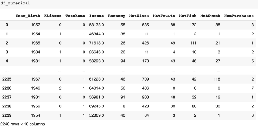All the columns are an numerical data type

Pandas Normalization

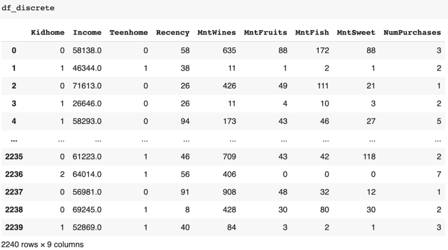
First, we take note of the columns that are finite, and countable. In our data, these are the Kidhome, Teenhome, Income, Recency, MntWines, MntFruits, MntFish, MntSweets, and NumPurchases columns.

Once we have the data we want, we can begin normalizing it following the equation.

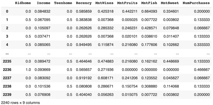After normalizing, the data should range from [0,1]

The results don’t look the best, some values like Kidhome and Teenhome turned out to lack in variance. In this case, we can repeat scaling but with standardization.

Pandas Standardization

All numerical columns can be standardized, so we’ll be looking at all of the data. Following the equation for standardization, we take the value, subtract it by the mean, then divide by the standard deviation.

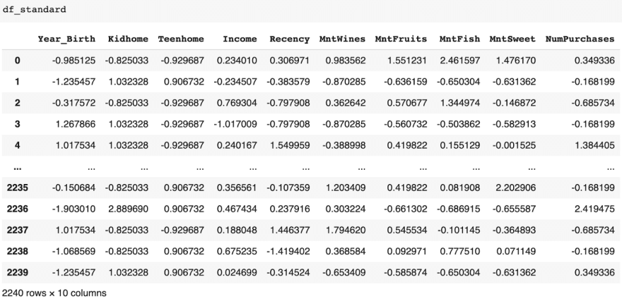Standardization has no range, but tries to fit in on a bell curve

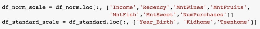
Based on the results, creating the best scaled dataset would take a combination of the results from normalization and standardization. We’ll start by concatenating the values from the df_norm that had low variance, then the remainder of numerical columns from df_standard. So we take the Year_Birth, Kidhome, and Teenhome columns from df_standard, and concat them with Income, Recency, MntWines, MntFruits, MntFish, MntSweet, and NumPurchases columns from df_norm.

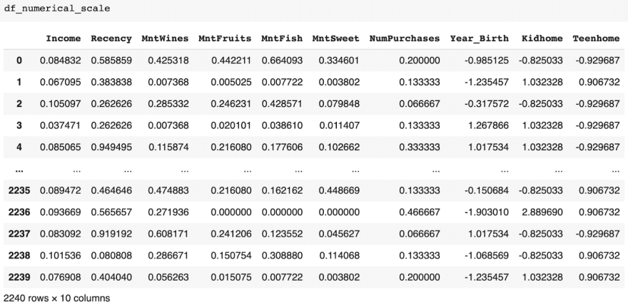
Our fully scaled numerical data

Use of Numerical Data

Machines like numbers a lot, and while humans aren’t able to understand what the 1’s and 0’s represent, they can still define what it means. Likewise, as numbers increase towards infinity, the meaning behind it is blurred for both humans and machines alike. On the other hand, you may want to create a ranking system in place to find out which customers are bringing in the big bucks. All this big data is useful in developing a machine learning model that can rank each of your customers and find out patterns hidden within the data. You’ve converted all the big data, but is all of that data necessary to train a good model? In our next part, we’ll look at how to impute data to clean the data further.