Conway's Game of Life, sparse

Introduction

A lot has been written about Conway's Game of Life. If you're reading this, chances are you've implemented a version of it yourself.

This article offers a visual guide to a less-common formulation of the game and presents a surprisingly succinct implementation of it, mostly for fun.

I'll assume you're already familiar with the game. If that's not the case, I'd recommend reading the original article published on Scientific American in 1970.

Canonical formulation

When you think of Game of Life, you probably think about a grid where live and dead cells are represented with different colors, and the following 3 rules define how to evolve the grid from the current state to the next (source: Wikipedia).

1. Any live cell with two or three live neighbours survives.
2. Any dead cell with three live neighbours becomes a live cell.
3. All other live cells die in the next generation. Similarly, all other dead cells stay dead.

These rules emphasise the role of both live and dead cells and lead to a straight-forward implementation where the state of the system is represented by a matrix of boolean values where each (i, j) entry represents a cell's state: true for live, false for dead.

A sparse formulation

Compact as the above might be, I've always found the following, equivalent formulation more interesting.

Consider an infinite grid of cells defined as per the canonical formulation. For each live cell, gather the coordinates (i, j) of all the cell's neighbours, plus the coordinates of the live cell itself.

Now count the number of times each cell appears in the collection.
Only the cells abiding by the following rules will be part of the next generation:

1. Any cell that occurs 3 times
2. Any cell that occurs 4 times and is currently live.

One thing I enjoy about this formulation, is the fact that it leads to a very natural implementation based on a sparse representation of the grid, where we only keep track of live cells.

Given a set of live cells - aptly called population - the next generation can be computed as follows - the code below is in Crystal, but your favourite language's implementation shouldn't differ much from this.

population.flat_map { |cell| expand(cell) }
  .tally
  .select { |cell, count| count == 3 || (count == 4 && population.includes?(cell)) }
  .keys

Here, expand is a simple function that returns the 9 cells in the 3x3 square centered in the cell passed as argument.

OriginSquare = [
  {-1,  1}, {0,  1}, {1,  1},
  {-1,  0}, {0,  0}, {1,  0},
  {-1, -1}, {0, -1}, {1, -1}
]

def expand(cell)
  OriginSquare.map { |(x, y)| {cell[0] + x, cell[1] + y} }
end

Let's explore the code line by means of an example.

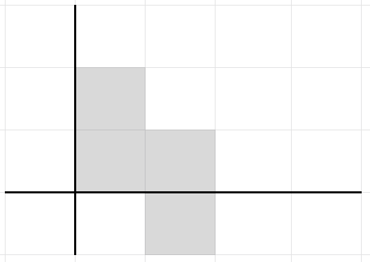
Consider the L-shaped population

population = [{2, 0}, {1, 0}, {0, 0}, {0, 1}]

We iterate over the live cells and expand them into the neighbouring cells plus the live cell itself - see Figure 2 below.

population.flat_map { |cell| expand(cell) }
# => [{-1, 2}, {0, 2}, {1, 2}, {-1, 1}, ..., {2, -1}, {3, -1}]

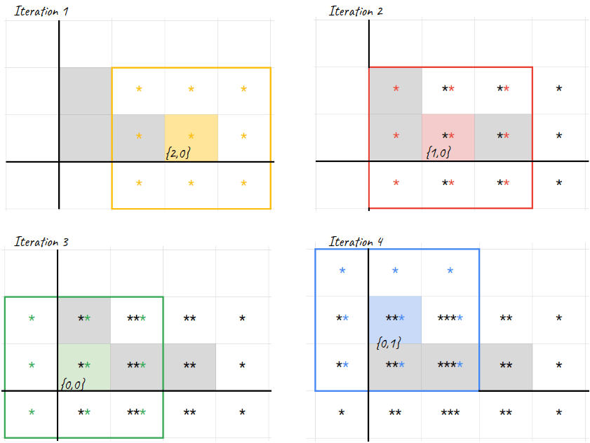
We now count the number of times a cell appears in the computed collection. In Crystal, this is as easy as calling #tally on an array. This returns a dictionary from cell to number of occurrences.

population.flat_map { |cell| expand(cell) }
  .tally
  # => {{-1, 2} => 1, {0, 2} => 1, ..., {3, -1} => 1}

Finally, we filter out any cell that doesn't match either rule 1 or rule 2 defined above. This is done by invoking .select on the dictionary with a predicate representing the rules.

population.flat_map { |cell| expand(cell) }
  .tally
  .select { |cell, count| count == 3 || (count == 4 && population.includes?(cell)) }
  # => {{0, 1} => 3, {0, 0} => 3, {1, 0} => 4, {1, -1} => 3}

We now discard the number of occurrences, and keep the cells' coordinates.

population.flat_map { |cell| expand(cell) }
  .tally
  .select { |cell, count| count == 3 || (count == 4 && population.includes?(cell)) }
  .keys
  # => [{0, 1}, {0, 0}, {1, 0}, {1, -1}]

Excellent! Let's talk about some of the features of this algorithm, but first...

Challenge. Now that we've discussed a script to evolve a population, can you extract this into a function or instance method, so that we can run an arbitrary number of evolutions? I'm thinking about something like

new_population = GameOfLife.evolve(population, times: 20)

Some notes on efficiency

The memory-efficiency of the sparse implementation makes evolving some configurations feasible, where they wouldn't be on the dense one. In particular, we can cope with cells patterns moving arbitrarily far from each other without going out of memory. This is not true for the dense implementation, where an initial population featuring, for example, two spaceships heading in different directions will exhaust your memory fairly quickly.

I like how the sparse implementation encodes a strong system invariant: in terms of state, nothing can ever change far from live cells.

Hence, the sparse implementation is more memory-efficient than the dense one, but the battle for best performance is totally open and depends on the configuration we're evolving. If you're thinking that the dense implementation might enjoy performance gains thanks to GPU architectures, then you're right on point.

Challenge. No matter the underlying implementation, printing a grid on the screen still poses a challenge, as we're materialising a possibly very large grid of cells. Can you think of strategies to display the current state of the grid that don't require printing it in its entirety?

Further reading

• In case you missed it, here is the original article where Conway's Game of Life was introduced.
• Towards data science offers an exhaustive coverage of both dense and sparse implementations of Conway's Game of Life in Python and in Haskel.
• If you'd like to know more about the Crystal programming language, then you can check out this page.

Thanks for reading, I hope this article made you want to sprint to your laptop and code the sparse Game of Life in your favourite language. You can share your Game of Life implementation in the comments section below, I'd love to see what you came up with.

If you'd like to stay in touch, then subscribe or follow me on Twitter.

This post was originally published on lbarasti.com.