
Optimizer is probably the most important piece of neural network because without a good optimizer it's not going to learn anything. Optimizer's job is to update parameters in a way that the model learns. The best optimizer reduces the loss quickly and doesn’t get stuck to any local optimal.
The code below is taken from this article I wrote about neural networks from scratch but to make it cleaner I turned it into a class. To make optimizers work with this class simply, I added a few new lines. I recommend to first check the optimizers before trying to understand this class fully.
class model:
    def __init__(self, x, y):
        self.x = x
        self.y = y

        self._initalize_parameters()
        self._initalize_moms()
        self._initalize_RMSs()

    def _initalize_parameters(self):
        self.weights_1 = self._random_tensor((x.shape[1],3))
        self.bias_1 = self._random_tensor(1)
        self.weights_2 = self._random_tensor((3,1))
        self.bias_2 = self._random_tensor(1)

    def _random_tensor(self, size): return (torch.randn(size)).requires_grad_()

    def _initalize_moms(self):
        self.moms_w1, self.moms_b1 = [0], [0]
        self.moms_w2, self.moms_b2 = [0], [0]

    def _initalize_RMSs(self):
        self.RMSs_w1, self.RMSs_b1 = [0], [0]
        self.RMSs_w2, self.RMSs_b2 = [0], [0]

    def _nn(self, xb):
        l1 = xb @ self.weights_1 + self.bias_1
        l2 = l1.max(torch.tensor(0.0))
        l3 = l2 @ self.weights_2 + self.bias_2
        return l3

    def _loss_func(self, preds, yb):
        return ((preds-yb)**2).mean()

    def train(self, optimizer):
        # Multiple learning rates to see how optimizers work with them
        lrs = [10E-4,10E-3,10E-2,10E-1]
        ## for plotting ##
        fig, axs = plt.subplots(2,2)
        ## for plotting ##
        all_losses = []
        for i, lr in enumerate(lrs):
            losses = []
            while(len(losses) == 0 or losses[-1] > 0.1 and len(losses) < 1000):
                preds = self._nn(self.x)
                loss = self._loss_func(preds, self.y)
                loss.backward()

                optimizer(self.weights_1, lr, self.moms_w1, self.RMSs_w1)
                optimizer(self.bias_1, lr, self.moms_b1, self.RMSs_b1)
                optimizer(self.weights_2, lr, self.moms_w2, self.RMSs_w2)
                optimizer(self.bias_2, lr, self.moms_b2, self.RMSs_b2)

                losses.append(loss.item())
            all_losses.append(losses)

            ## for plotting ##
            xi = i%2
            yi = int(i/2)
            axs[xi,yi].plot(list(range(len(losses))), losses)
            axs[xi,yi].set_ylim(0, 30)
            axs[xi,yi].set_title('Learing Rate: '+str(lr))
            ## for plotting ##

            # Setting seed makes sure the parameters are
            # initalized the same way for better comparison
            torch.manual_seed(42)
            self._initalize_parameters()
            self._initalize_moms()
            self._initalize_RMSs()

        ## for plotting ##
        for ax in axs.flat:
            ax.set(xlabel='steps', ylabel='loss (MSE)')
        plt.tight_layout()
        ## for plotting ##
This time I needed more data so I created this simple function to generate y values from x values.
def generate_fake_labels(x3, x2, x1):
    return (x3**3 * 0.8) + (x2**2 * 0.1) + (x1 * 0.5) + 4.
x = torch.tensor([[0.7,0.3,0.7],
                  [0.4, 1., 0.4],
                  [0.2, 1.1, 0.1],
                  [0.4, 0.7, 0.2],
                  [0.1, 0.5, 0.3]])
y = torch.tensor([generate_fake_labels(i[0],i[1],i[2]) for i in x])
print(x.shape, y.shape, y)

CONSOLE: (torch.Size([5, 3]),
          torch.Size([5]),
          tensor([4.6334, 4.3512, 4.1774, 4.2002, 4.1758]))
y could have been also initialize manually.
y = torch.tensor([4.6334, 4.3512, 4.1774, 4.2002, 4.1758])
The last "get started" thing to do is to use the class defined above to create a model.
my_model = model(x, y)
Vanilla SGD
Stochastic gradient descent is the base in the most used modern optimizers. Stochastic version of gradient descent is just calculating gradient using mini-batch (subset of data) instead of the whole dataset.
In vanilla SGD parameters are updated by subtracting gradient times learning rate from parameters.
def SGD(a, lr, _, __):
    a.data -= a.grad * lr
    a.grad = None
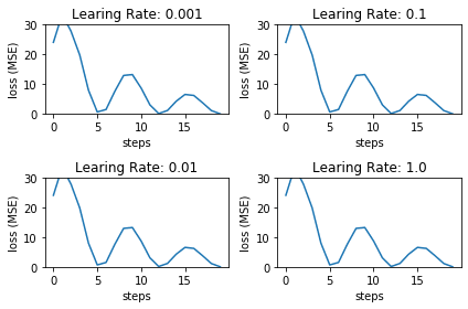
my_model.train(SGD)

Momentum
In vanilla SGD there is a problem that steps continue to be small even though the model might be pretty sure that the direction is right. Momentum takes bigger and bigger steps the more sure it is about the direction.
In momentum optimizer we need to first calculate momentum. It's gradient times small value (almost always 0.1) multiplied by previous momentum times 1-the_small_value. This way it mostly goes to the same direction where it was going the last time but gradient still can change the direction.
def momentum(a, _, moms, __):
    previous_momentum = moms[-1]

    mom = a.grad * 0.1 + previous_momentum * 0.9
    moms.append(mom)
    a.data -= mom
    a.grad = None
my_model.train(momentum)
RMSprop
RMSprop is the same as momentum except gradient is squared.
Because the gradient is squared it means that if the gradient is:
- small RMSprop becomes small
- volatile RMSprop becomes big
- big RMSprop becomes big
Then parameteres are updated by multiplying the gradient with learning rate and then dividing it with square root of RMSprop. This means that if RMSprop is small the parameters are updated more.
def RMSprop(a, lr, _, RMSs):
    previous_RMS = RMSs[-1]

    RMS = (a.grad ** 2 * 0.1 + previous_RMS * 0.9)
    RMSs.append(RMS)
    # Gamma is added to make sure there is never divide with zero
    gamma = 1E-5
    a.data -= (a.grad * lr) / (torch.sqrt(RMS) + gamma)
    a.grad = None
my_model.train(RMSprop)

Adam
Adam is simply combination of RMSprop and momentum. That's it. Nothing more. Adam is often the safe choice in any model even though some other optimizer might be better in specific tasks.
def Adam(a, lr, moms, RMSs):
    previous_momentum = moms[-1]
    mom = a.grad * 0.1 + previous_momentum * 0.9
    moms.append(mom)

    previous_RMS = RMSs[-1]
    RMS = a.grad ** 2 * 0.1 + previous_RMS * 0.9
    RMSs.append(RMS)

    gamma = 1E-5
    a.data -= (mom * lr) / (torch.sqrt(RMS) + gamma)
    a.grad = None
my_model.train(Adam)

One thing to notice about these experiments is that I used artificial and small dataset. In more complex datasets it's easier to see the differences more clearly but after a long thinking I decided to use this simple data to make it easy to understand. With this small dataset it’s possible to print the gradients and other values for better understanding.
To continue this further one very common thing is to reduce learning rate as the loss start to drop because right now in some plots it’s possible to see how the loss stays very small but never goes to zero. But that's another topic to cover someday. If interested to dig deeper after understanding this I highly recommend this amazing article by Sebastian Ruder. or it's sequel.
I decided to use PyTorch in this article when the last time I created PyTorch and Tensorflow versions. For me both libraries are fine and I don’t have any preference over other as they are very similar. If you have a preference for either library (or some other) and wish me to use it, please leave a comment below and I will count how many wants Tensorflow vs. PyTorch and use winner the next time.

Top comments (0)