Massively Parallel Fun with GPUs: Accelerating Tensors in Rust

In this second installment of Tensors from Scratch, I'll walk through an implementation of tensor operations on the GPU using wgpu. Wgpu is a Rust implementation of the WebGPU working draft standard, which aims to make GPUs accessible to browsers.

I'll build on the CPU implementation of tensors from the first post, in the aspirational tensor library I'm building called Tensorken. All code for Tensorken is on GitHub. The version this post discusses is tagged v0.2, and all links are to that version.

I'm not assuming any knowledge of GPU programming, which is the state I started from before I wrote all this. I do assume proficiency with programming on the CPU, aka typical software engineering experience. As usual, some Rust experience is helpful but not strictly necessary.

First, I'll recap some tensor-related terms and basic tensor operations introduced in the last post. This post implements those same operations on the GPU, parallelizing them. As a result, they'll execute much quicker than my earlier, admittedly naïve CPU implementations. Feel free to skip the recap if you don't need the refresher.

This post introduces a new set of GPU-related terms, explains how GPUs work on a high level and meanders to a well-known parallel programming building block, the parallel prefix sum. Brace yourself for a long read!

Previously in Tensors From Scratch: neural networks and matrix multiplication

Last time, I argued that neural networks don't have much to do with either neurons or networks. Modern neural networks, for example large language models (LLMs) like OpenAI's ChatGPT and GPT-4, Microsoft's Bing, Google's Bard, and Anthropic's Claude, are powered by tensors. Tensors are multi-dimensional arrays augmented with powerful operations that execute remarkably efficiently on modern hardware, most notably GPUs.

To understand all that, I intend to build a neural network library like PyTorch or JAX, in Rust, from the ground up. While these libraries are gazillions of lines of code each, they consist of the following parts:

1. A tensor library, to provide efficient operations to slice, dice, and apply bulk operations to tensors.

2. Accelerators, to execute tensor operations on the GPU, accelerating them greatly.

3. Automatic differentiation, to efficiently train neural networks via gradient descent.

4. Neural network building blocks, to easily reuse commonly used activation functions and layers.

In the first post, I focussed on the tensor library. I described almost twenty fundamental tensor operations and abstracted them in a Rust trait called RawTensor. This trait had a single implementation, CpuRawTensor.

The fundamental tensor operations can be categorized as follows:

1. Unary operations take a single tensor as input and produce a new tensor of the same shape, by applying a function to each element: log and exp.

2. Binary operations take two tensors as input and produce a new tensor of the same shape, by applying a binary function element-wise: add, sub, mul, div, pow and eq.

3. Reduce operations take a tensor as input, and produce a new tensor of a smaller shape, by reducing one or more dimensions to length 1. These are sum and max.

4. Movement operations take a tensor as input, and produce a new tensor with a changed shape, without changing its elements. These are reshape, permute, expand, pad, and crop.

5. Creation and elimination operations make and destroy tensors. These are new, shape and ravel.

To prove that these operations are necessary and sufficient, we implemented matrix multiplication using only RawTensor operations:

1. massage the left tensor with shape (m, n) to shape (m, 1, n), using reshape.

2. massage the right tensor with shape (n, o) to shape (1, o, n), using reshape and permute.

3. broadcast-multiply left and right to make a tensor of shape (m, o, n) using expand, reshape, and mul.

4. reduce the last dimension to make a tensor of shape (m, o, 1) using sum.

5. reshape to (m, o).

So far the recap, on to the main event.

GPU and me

You only have to look at NVIDIA's stock price to see that GPUs and neural networks go hand in hand. Not surprising in hindsight: the main computational load of neural networks is a bunch of linear algebra operations, and the main computational load of "showing 3D shapes on a 2D screen" is definitely in the same ballpark, if not the same ball.

Think of your GPU as the supercomputer you never knew you had. Did you ever wonder why you can play Fortnite at 60 fps, moving around fluidly in a multiplayer 3D world with a UI overlay, while online banking takes more than 30 seconds to display a few static numbers? That's because your GPU is amazingly good at its job.

To drive this point home, let's compare my CPU with my GPU in units of peak floating point operations per second (FLOPS). The comparison is not necessarily apples to apples, and there are various problems with calculating such peak performance and how realistic it is. I'm just going to ignore that.

I bought a mid-to-high-end laptop 2.5 years ago. It has an Intel Core i7-10750H, which Intel reports has 249.6 GFLOPS (that's Giga FLOPS) peak performance. It's unclear whether that's for single (f32) or double (f64) precision. I suspect it's f32, but let's be generous and say it's f64, and assume single precision is twice as fast. Then my CPU can add f32s at a cool 500 GFLOPS.

My laptop has an NVIDIA GeForce RTX 2070 (released Oct 2018) GPU with a peak performance of 7.465 TFLOPS for f32. Yes, that's "T" for Tera.

Here, let me put that in a pie chart for you:

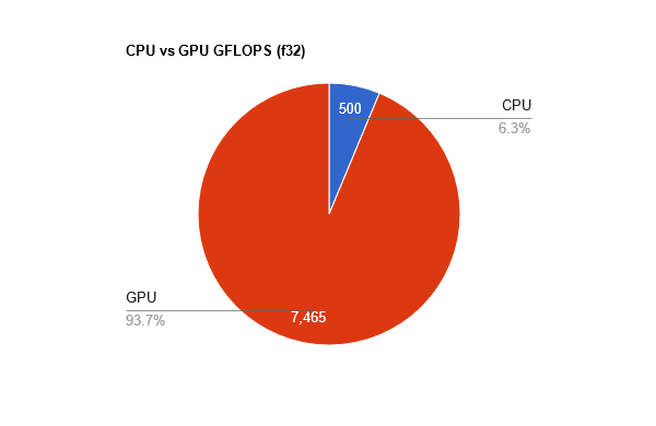
"But but but!" I hear you say. "According to that page, your GPU only has a peak performance of 233 GFLOPS for f64, which is LESS than your CPU." That's right. GPUs are optimized for f16 and f32 operations. You'll also notice that my GPU's f16 performance is twice as fast as f32 performance, while f64 is 32 times as slow. That's because f32 is plenty for graphics and neural network applications. People are getting good results with stuffing the numbers in 8 or even 4 bits. While that needs clever engineering, floating point precision does not seem to be a limiting factor.

You want the threads? You can't handle the threads

GPUs achieve such high FLOPS by massive parallelization.

On the most fundamental level, they have built-in instructions that execute vector or matrix operations in a single cycle. For example, NVIDIA's Turing architecture GPUs include so-called tensor cores. My RTX 2070 has 288 of them. These cores are specialized to execute General Matrix Multiplication or GEMM. GEMM computes the result of 𝙰×𝙱+𝙲, a fused multiply-add operation. Each tensor core executes 64 GEMMs per clock cycle on 4×4 matrices containing f16s. NVIDIA writes: "Tensor Cores are specialized execution units designed specifically for performing the tensor/matrix operations that are the core compute function used in Deep Learning. " This is from a post written in 2018. Their recent stock price explosion isn't entirely out of the blue.

On top of that, GPUs expose more parallelism using threads. GPU threads are more limited than the threads you are probably thinking about. For example, small groups of threads may share the same stack and so must all execute the same code. Threads execute in workgroups, groups of threads that share a fast cache. Using this shared cache well is often critical for performance. On modern GPUs, 100s or 1000s of threads are available in execution units like tensor cores.

Launching workgroups for execution on the GPU is called dispatching or a dispatch. The GPU driver schedules workgroups for execution, similar to how an operating system's kernel schedules processes. A single dispatch in WebGPU can launch up to 65,535³ threads, divided into workgroups of up to 256 threads each.

The technical term for this is a fucktonofthreads.

Everything, everywhere, all at once

Like any subfield, GPU programming has a set of terms that takes some time to get used to. I've introduced thread, workgroup, and dispatch already. Unfortunately, different hardware vendors or graphics APIs use other terms for essentially the same thing or the same terms for subtly different things! Since I'll use WebGPU, I use their terminology exclusively. Raph Levien has put together a useful Compute Shader Glossary.

I will focus on concepts, and leave the details of APIs to others. Also, I will not explain and frankly do not know how to do graphics programming on the GPU.

GPUs, like CPUs, execute code, so the first order of business is writing a program that compiles to whatever GPUs execute. For historical reasons, these programs are called compute shaders. In the original graphics context, they were simply called shaders. The compute emphasizes that the shader is a general computation, that doesn't show things on the screen.

Shaders are written in a domain-specific shading language. Most shading languages have a C or C++-like syntax. WebGPU's Shading Language, or WGSL, has a Rust-like syntax. To do you a flavor, here's a shader entry point, like a main function, in WGSL. Don't worry about what this does for now.

@compute
@workgroup_size(64)
fn call(@builtin(global_invocation_id) global_id: vec3<u32>) {
    let fro = global_id.x * strides_and_shape[2];
    let to = fro + strides_and_shape[2];
    for (var gidx = fro; gidx < to; gidx = gidx + 1u) {
        let index = input_index_of(gidx);
        output_0[gidx] = log(input_0[index]);
    }
}

For CPUs, compilers like gcc take program text and compile it to a well-defined instruction set like x86. For GPUs, the situation is more complicated. Even GPUs produced by the same vendor like NVIDIA, don't all have the same instruction set. To avoid application programmers having to learn the interface of all GPU cards out there, a graphics API mediates between the programmer and the hardware. You've almost certainly heard about graphics APIs: Direct3D 12 on Windows, Metal on Apple, Cuda for NVIDIA chips, Vulkan, and WebGPU. The GPU driver, written by the manufacturer, bridges the gap between the hardware and the graphics API, and the graphics API is what programmers use.

As you can see from the examples, this doesn't make the situation comparable to CPUs, as even on the graphics API level you still have to pick a platform or manufacturer. Wgpu addresses this to some extent: it's not a standalone graphics API, but a layer that interfaces with actual graphics APIs. You can take a shader written in WebGPU's WGSL and run it on a Vulkan backend or a DirectX backend, all from the wgpu API, without changing any code. Wgpu uses a library called naga to translate shaders in WGSL and other supported shading languages to the desired shading language.

Compared to CPUs, the graphics API is in some sense the GPU's operating system and compiler in one. It is responsible both for compiling shader code and scheduling the resulting program for execution on the GPU.

The final piece of the puzzle is memory. Discrete GPUs, which come on a separate card, have dedicated memory onboard. Since GPUs are so highly parallelized, there must be enough memory bandwidth available, and having to copy over a PCI bus from main memory just doesn't cut it. GPU memory is not accessible by the CPU, but like other devices, the GPU can access shared memory on the CPU. Shared memory is used as a staging area: you fill buffers in shared memory and instruct the GPU to copy to its memory or do the same in reverse to get data from GPU to shared memory.

That's pretty much it. You start a GPU program by setting up the buffers it needs to read and write, pointing at the shader code that needs to run, and dispatch it by giving the number of workgroups you'd like to run. The graphics API does the rest and notifies you when the GPU is done with your dispatch. From the main program's perspective, which runs on the CPU, this all happens asynchronously.

So much for the high-level overview. As we'll find out, the details matter a lot!

In the rest of this post, I'll describe an implementation of raw tensor operations on the GPU using WebGPU. I picked WebGPU because it sounded like the easiest-to-understand API while remaining low-level and cross-platform.

As the name indicates, in principle WebGPU is executable entirely in the browser via WASM. However, WebGPU is an emerging standard, not an established implementation. While WebGPU is supported by all the important browser creators (Apple, Mozilla, Google, Microsoft), as of June 2023 it's not available by default in any major browser. The implementation in Chrome, called Dawn, is the closest. You can enable it using a special flag. The implementation for Firefox is called wgpu, and it's available behind a flag in nightly builds.

However, both Dawn and wgpu are available as standalone libraries. Dawn is written in C++ and wgpu in Rust. So, wgpu is a natural target for this series.

There are already good quality posts out there that tell you how to get started with wgpu, and explain the details of the wgpu API. I'll gloss over those. Instead, I'll try to explain the underlying concepts which also transfer to other GPU programming APIs.

Wgpu 101: Accelerating unary operations

Let's dip our toes in GPU programming by implementing the unary tensor operations, as defined in RawTensor:

fn exp(&self) -> Self;
fn log(&self) -> Self;

These two operations apply the exp and log functions to each element in the tensor.

Recall that a tensor is backed by a 1-dimensional array. On the CPU, the implementation of exp and log is straightforward: allocate a new result buffer, loop over each element in the original buffer, and store the result in the result buffer. Unary operations can be optimized easily, for example via multithreading and SIMD instructions. I've done no optimization whatsoever. The idea is to compare a naïve CPU implementation with a naïve GPU implementation, and pretend that's apples-to-apples.

CpuRawTensor is a struct defined as:

pub struct CpuRawTensor<T> {
    buffer: Arc<Buffer<T>>,
    strider: ShapeStrider,
}

It contains a reference-counted buffer, and a ShapeStrider which is responsible for translating multi-dimensional tensor indices to a one-dimension buffer index. The buffer is reference-counted because it's immutable and can be shared: operations like reshape and permute only change the shape or the strides of the tensor.

The definition of WgpuRawTensor is remarkably similar:

pub struct WgpuRawTensor<'a, T> {
    buffer: Arc<wgpu::Buffer>,
    strider: ShapeStrider,
    context: &'a WgpuContext,
    phantom: std::marker::PhantomData<T>,
}

Again we have a buffer, but here it lives in GPU memory. We also have ShapeStrider for the same reasons we have one on the CPU: movement operations don't usually touch the buffer, and they are almost identical to the CPU implementation. ShapeStrider lets us share that code.

The other fields are WgpuContext to facilitate interaction with Wgpu's API and keep some state that's shared among all tensors. Finally, since Wgpu's buffer is not typed, PhantomData<T> keeps Rust's type system happy.

Now onto implementing our first shader. Let's simplify further and assume we're writing a shader for exp only.

@group(0) @binding(0)
var<storage, read> input_0: array<f32>;

@group(0) @binding(1)
var<storage, read_write> output_0: array<f32>;

@compute
@workgroup_size(64)
fn call(@builtin(global_invocation_id) global_id: vec3<u32>) {
    let gidx = global_id.x;
    output_0[gidx] = exp(input_0[gidx]);
}

The most familiar pieces here are:

• Definitions of input_0 and output_0 buffers for the shader to read from and write to.

• A function call as the entry point of the shader.

• The last line of the shader reads a value from the input buffer at index gidx, applies the built-in exp function, and writes the result to the output buffer at gidx.

One mystifying aspect is that there's no loop: this program only updates a single index. The secret sauce here is threads. We'll dispatch as many threads as there are elements in the output buffer, so each thread reads a single element of the input and writes a single element to the output.

How does a thread know which index it should write to the output? That's where the @builtin(global_invocation_id) attribute comes in. A shader entry point like call is limited in the arguments it can accept. To my knowledge, a compute shader can only accept invocation ids, which are set by the graphics API. The shader entry point is called N times, on N different threads, and each of these threads gets a unique invocation id, with 0 <= id < N. The shader above uses this invocation id to figure out which index a thread should process. It's important to keep different threads from writing to the same location because that creates a race condition.

In principle, that's the end of the story, but for a mix of historical and performance reasons, it is complicated further. First, the invocation id is not a single number: it's a vec3 type, a coordinate (x, y, z). I can imagine this is because of roots in 3D graphics, although some material also implies that threads that are nearby in coordinate space are located close together (e.g. neighboring GPU cores or the same core), while others imply that for modern GPUs this isn't so much the case anymore. I'm only using the x-coordinate anyway, so you can think of the invocation id as a single number.

A further complication comes with the organization of GPU threads into workgroups. The wgpu API doesn't let you specify how many threads you want. Instead, you specify how many workgroups you want:

/// Dispatches compute work operations.
///
/// `x`, `y`, and `z` denote the number of work groups to dispatch in each dimension.
pub fn dispatch_workgroups(&mut self, x: u32, y: u32, z: u32)

The @workgroup_size attribute in the shader specifies how many threads each workgroup has. You may wonder why everything has an (x, y, z) coordinate except @workgroup_size. It does, but any omitted dimensions default to 1. So I could also have written @workgroup_size(64, 1, 1).

The idea is that threads in the same workgroup share fast cache memory and can coordinate, for example via barriers that wait for all threads in a workgroup to reach a certain point. Workgroups on the other hand may or may not run concurrently, depending on how they are scheduled by the GPU driver. There are no WGSL operations that allow coordination between threads in different workgroups.

What this means in practice is that a shader with an attribute @workgroup_size(wx, wy, wz) and dispatched using dispatch_workgroups(cx, cy, cz) executes the entry point wx × wy × wz × cx × cy × cz times, and each of those threads gets a unique invocation id (x, y, z).

The remaining bit I haven't explained yet is the declaration of the storage buffers:

@group(0) @binding(0)
var<storage, read> input_0: array<f32>;

@group(0) @binding(1)
var<storage, read_write> output_0: array<f32>;

They're familiar arrays of f32. But what's the var stuff between the angle brackets? WGSL partitions memory in address spaces. Address spaces are like a type of memory with specific properties. These properties determine mutability, visibility, the type of values that may be stored, and how to use the variables. For now, we'll only use the storage address space, which is for buffers provided when dispatching the computation. These buffers are visible to all threads in the dispatch and can be read-only or read-and-write. The other address space we'll use later is workgroup, declared as var<workgroup>, which is for buffers that are shared between threads in the same workgroup.

The @group and @binding attributes identify which buffers to bind before dispatching. On the Rust side, we need to specify a bind group that matches the definition in the shader:

// get bind group 0 = all the bindings with @group(0)
let bind_group_layout = pipeline.get_bind_group_layout(0);
// index 0 and 1 within group 0, for the input and output buffer (which are wgpu::Buffer types)
self.device().create_bind_group(&wgpu::BindGroupDescriptor {
    label: None,
    layout: &bind_group_layout,
    entries: &[
        wgpu::BindGroupEntry {
            binding: 0,
            resource: self.buffer.as_entire_binding(),
        },
        wgpu::BindGroupEntry {
            binding: 1,
            resource: output_buffer.as_entire_binding(),
        },
    ],
})

The last bit of admin in the shader is the @compute annotation. I've mostly pretended there's only one type of shader, the compute shader. There are other kinds of shaders specific to graphics computations, like @vertex and @fragment. You can think of those as more specialized compute shaders, although historically they predated them. I'll continue to ignore these other shader types. You may want to look into them if you're interested in graphics programming.

Can we run something now?

Pretty much! There is a bunch of wgpu-specific admin I cover briefly here. Feel free to skip this section.

Wgpu's entry points are Device and Queue. The device represents the logical GPU and has functions for creating compute resources, like buffers and compiled shaders. The queue enqueues commands for the GPU to execute. The only commands I've used are for dispatching a shader and copying buffers from shared memory to GPU memory. Once submitted, the GPU works through them, and you can poll for completion asynchronously.

I've created a Device and Queue lazily, and once per process, then pass a singleton WgpuContext to every WgpuRawTensor instance:

pub(crate) struct WgpuContext {
    pub(crate) device: wgpu::Device,
    pub(crate) queue: wgpu::Queue,
    pipelines: RwLock<HashMap<(&'static str, WorkgroupSize), Arc<wgpu::ComputePipeline>>>,
}

This brings us to ComputePipeline. A compute pipeline contains a compiled and validated shader, with some information like the name of its entry point. You create it via wgpu::Device.create_compute_pipeline. Since parsing, compiling, and validating the shader takes time, WgpuContext contains a cache of created pipelines. A pipeline can be re-executed as many times as desired.

Once you have your shader code, executing the shader proceeds as follows:

1. Create any necessary buffers, and copy data to them via functions on wgpu::Device.

2. Create the ComputePipeline for the shader.

3. Bind buffers from step 1 to corresponding variables defined in the shader via bind groups. Bind groups are created via wgpu::Device.

4. Dispatch the shader with a given number of workgroups. This step is somewhat tedious, and needs a few intermediate objects like a "command encoder" and a "compute pass". The gist is you submit a list of commands to the Queue, and get a submission index back.

5. Poll the device using this submission index, to learn when execution finishes.

256 by 256 is enough for everyone

Now can we run something? Why yes, I thought you'd never ask.

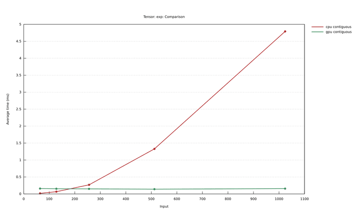
To compare my naïve CPU tensor implementation with my naïve GPU implementation, I set up a few benchmarks using criterion.rs. The benchmark creates random square tensors of various sizes (from 64x64 to 1024x1024) and then compares calling exp on the CPU (CpuRawTensor) with the GPU (WgpuRawTensor):

let mut rng = StdRng::seed_from_u64(12345u64);

for size in [64, 128, 256, 512, 1024] {
    let t1s = &[size, size];
    let t1_gpu = Wgpu32::randn(t1s, &mut rng);
    let t1_cpu = t1_gpu.to_cpu(); // copies the tensor from GPU to CPU memory

    group.bench_with_input(BenchmarkId::new("cpu contiguous", size), &size, |b, _| {
        b.iter(|| t1_cpu.exp())
    });
    group.bench_with_input(BenchmarkId::new("gpu contiguous", size), &size, |b, _| {
        b.iter(|| t1_gpu.exp())
    });
}

I've removed some criterion-related boilerplate to make it more readable.

When I run this, it fails. The maximum number of threads you can dispatch in a single call along a single dimension is 65k, and we're hitting that limit around size 256x256. Tensors used in neural networks today are bigger than that.

The solution is straightforward: instead of only a single element, each thread processes a few elements using a loop. Our shader becomes:

@group(0) @binding(0)
var<storage, read> input_0: array<f32>;

@group(0) @binding(1)
var<storage, read_write> output_0: array<f32>;

@group(0) @binding(3)
var<storage, read> chunk_size: u32;

@compute
@workgroup_size(64)
fn call(@builtin(global_invocation_id) global_id: vec3<u32>) {
    let fro = global_id.x * chunk_size;
    let to = fro + chunk_size;
    for (var gidx = fro; gidx < to; gidx = gidx + 1u) {
        if(gidx >= arrayLength(&output_0)) {
            return;
        }
        output_0[gidx] = exp(input_0[gidx]);
    }
}

I added another binding buffer to pass the chunk size to the shader. We'll expand it with more parameters soon. If the length of the output buffer is not evenly divisible by the chunk size, the last thread accesses an out-of-bounds array index. WebGPU clamps array indices, so it doesn't cause an error but leads to wrong results.

With that change, we have a working shader!

Comparing GPU vs CPU performance gives:

Making shaders generic

Besides exp, we'd like to apply log. We could copy-paste the shader and replace one word, but that doesn't work well if there are more parameters. In particular, we'd also like to modify the workgroup size: no use starting 64 threads per workgroup if a tensor has only 16 elements. (As a reminder, workgroup size is the number of threads per workgroup, not to be confused with the number of workgroups.) Because workgroup size is defined in the shader using the workgroup_size attribute, we'll need to munge some shader text if we want to make this parametrizable.

Simplicity is my main objective, so instead of string templating, I've gone for parlor tricks and string replacement. Let's update the shader again:

fn replace_me_with_actual_operation(in: f32) -> f32 { discard; }

@compute
@workgroup_size(64)
fn call(@builtin(global_invocation_id) global_id: vec3<u32>) {
    let fro = global_id.x * strides_and_shape[2];
    let to = fro + strides_and_shape[2];
    for (var gidx = fro; gidx < to; gidx = gidx + 1u) {
        if(gidx >= arrayLength(&output_0)) {
            return;
        }
        output_0[gidx] = replace_me_with_actual_operation(input_0[gidx]);
    }
}

The explicit call to exp is now a custom function we must replace before giving the shader to wgpu. The discard operation is a built-in not applicable to compute shaders. Leaving it in would cause an error, which is the point: it's an assert of sorts to check if string replacement has worked correctly. One advantage of not using templating is that syntax highlighting still works. VSCode has a decent language service addon for WGSL. It catches many errors beyond syntactic ones, so I was keen to keep it functional.

The Rust side now has to do a few string operations before passing the shader text to wgpu:

// include the shader text from a file
const MAP_SHADER: &'static str = include_str!("shaders/map.wgsl");
const REPLACE_OP_NAME: &'static str = "replace_me_with_actual_operation";
const REPLACE_UNARY_OP_DEF: &'static str =
    r"fn replace_me_with_actual_operation(in: f32) -> f32 { discard; }";
const REPLACE_WORKGROUP_SIZE: &'static str = "@workgroup_size(64)";

pub(crate) fn pipeline_for(
    &self,
    operation: &'static str,
    workgroup_size: WorkgroupSize,
) -> Arc<wgpu::ComputePipeline> {
    // snip
    &Self::MAP_SHADER
        .replace(Self::REPLACE_UNARY_OP_DEF, "")
        .replace(Self::REPLACE_OP_NAME, operation)
        .replace(
            Self::REPLACE_WORKGROUP_SIZE,
            &format!(
                "@workgroup_size({}, {})",
                workgroup_size.0, workgroup_size.1
            ),
    ),
    // snip
}

The first replace removes the replace_me_with_actual_operation function definition, the second replaces the call with the actual operation like exp or log, and the third puts in a given workgroup size. Note the workgroup size is in two dimensions - the second dimension is only used for reduce operations, as I'll describe below.

It's not the most beautiful code, but that comes with the territory.

Give yourself a pat on the back, you’ve reached the half-way point in the post!

Photo by Reiseuhu on Unsplash

Non-contiguous unary operations

Unary operations don't care if the tensor is non-contiguous: the result is correct either way. They don’t need to take the shape or strides of the tensor into account.

Interlude: Shape and strides reminder. Skip if you're familiar, or check out the last post if nothing makes sense.

• A tensor can have any number of dimensions or axes. Each axis is indexable, conventionally zero-based, and has a length.

• The shape of an n-dimensional tensor is an n-tuple of lengths for each dimension.

• The product of the lengths is the number of elements in the tensor - called the tensor's size.

• The strides of an n-dimensional tensor is an n-tuple that represents how many elements to skip in the underlying (one-dimensional) buffer to get to the next element in that dimension. Many movement operations, like reshape and permute, only need changes to shape and strides, which saves a copy of the underlying buffer.

• In general, the tensor's shape and strides represent a coordinate transformation from a many-dimensional tensor index to a one-dimensional buffer index.

In contrast, for non-unary operations, we'll have to take shape and strides into account. It's incorrect to add two tensors elementwise by adding pairs of elements in their underlying buffers. Unless they are both contiguous, we need to pair up elements according to the tensor index, not the buffer index.

For consistency, I decided to make the result of all operations contiguous, including unary operations. We'll have to modify the shader one last time. We'll no longer assume the input buffer is contiguous, and we must make the output buffer contiguous. All the rest remains the same: we'll divide the output buffer into chunks, and each thread writes only to the chunk it is responsible for.

The problem becomes: given an index in a contiguous output buffer, which is given via the invocation id, what is the corresponding index in the potentially non-contiguous input buffer? In the contiguous case, the index in the input is the same. In the non-contiguous case it depends on the shape and strides of the input tensor.

Here's the final code of the shader's entry point, call:

@compute
@workgroup_size(64)
fn call(@builtin(global_invocation_id) global_id: vec3<u32>) {
    let fro = global_id.x * strides_and_shape[2];
    let to = fro + strides_and_shape[2];
    for (var gidx = fro; gidx < to; gidx = gidx + 1u) {
        if(gidx >= arrayLength(&output_0)) {
            return;
        }
        let index = input_index_of(gidx);
        output_0[gidx] = replace_me_with_actual_operation(input_0[index]);
    }
}

This code first transforms gidx into the input buffer index by calling input_index_of, which I have yet to show.

To implement input_index_of, let's make the problem more precise. We have a mapping 𝚋 from an n-dimensional tensor index (𝚝₀, 𝚝₁, ..., 𝚝ₙ₋₁) in the input to its buffer index. Given n-dimensional shape (l₀, l₁, ..., lₙ₋₁) and strides (𝚜₀ , 𝚜₁ , ..., 𝚜ₙ₋₁):

𝚋(𝚝₀,𝚝₁,...,𝚝ₙ₋₁) = ∑ᵢ 𝚜ᵢ⋅𝚝ᵢ

This mapping is defined by the input tensor's shape and strides. Similarly, we have the shape and strides of the output tensor: the shape is identical to the input tensor, and the strides are chosen to make the tensor contiguous.

The mapping 𝚋 is reversible. From a buffer index 𝚎, we can back out the corresponding tensor indices (𝚝₀, 𝚝₁, ..., 𝚝ₙ₋₁):

𝚋⁻¹(e) = (..., (𝚎 ÷ sᵢ) % 𝚕ᵢ, ... )

The reverse mapping is what we need because we have the output buffer index as a given: it's gidx. We can back out the output buffer's tensor index by applying 𝚋⁻¹ with the shape and strides of the output buffer. The input tensor index is identical to the output tensor index because unary operations map element by element. So to get the input buffer index we apply 𝚋 with the input tensor's shape and strides to the tensor index we obtained from the reverse mapping. In short, input_index_of calculates:

𝚋ᵢₙ (𝚋ₒᵤₜ⁻¹ (e))

In code:

// ndims, input_offset, chunk_size, input_strides, output_strides, shape
@group(0) @binding(2)
var<storage, read> strides_and_shape: array<u32>;

const preamble: u32 = 3u;

fn input_strides(i: u32) -> u32 {
    return strides_and_shape[i + preamble];
}

fn output_strides(i: u32) -> u32 {
    return strides_and_shape[i + preamble + strides_and_shape[0] ];
}

fn shape(i: u32) -> u32 {
    return strides_and_shape[i + preamble + strides_and_shape[0] * 2u];
}

fn input_index_of(output_i: u32) -> u32 {
    let ndims = strides_and_shape[0];
    let offset = strides_and_shape[1];

    var input_i: u32 = offset;
    for (var i: u32 = 0u; i < ndims; i = i + 1u) {
        let len = shape(i);
        let stride = output_strides(i);
        let coord_i: u32 = output_i / stride % len;

        input_i += coord_i * input_strides(i);
    }

    return input_i;
}

I've added a third binding with an array that contains the necessary dimensions, shapes, and strides for the coordinate transformations. It also contains the chunk size which we added earlier. WGSL has structs, but a struct can only contain a dynamically sized array as its last element, so it was little help here. Instead, I've just plonked everything in a single array and created a few helper methods to keep things civilized.

The implementation avoids an intermediate tensor index representation by calculating dimension by dimension. I don't think it's possible in WGSL to have an explicit representation because local, dynamically sized array variables are not allowed.

Now that we can produce contiguous tensors from non-contiguous tensors, let's benchmark if this slows us down. I added a few reshaped and transposed tensors to the benchmark:

let t1_gpu = Wgpu32::randn(t1s, &mut rng);
let t1_gpu_nc = t1_gpu.reshape(&[size / 2, size * 2]).transpose(0, 1);
let t1_cpu = t1_gpu.to_cpu();
let t1_cpu_nc = t1_gpu_nc.to_cpu();

Running the exp operation on these four tensors, for the same sizes I showed earlier.

Not sure what I was expecting, but no significant difference works for me!

Binary operations

Implementing a shader for binary operations is straightforward now that we know how to implement the coordinate mapping. The entry point for the shader looks almost identical, except that the binary operation takes two arguments. It also takes an extra input buffer for the second input tensor. What's cute is that input_index_of is also nearly identical. We just need to use a vec2<u32>, a pair of u32 numbers, instead of a simple u32 to calculate the buffer indices in both input buffers at the same time:

fn input_index_of(output_i: u32) -> vec2<u32> {
    let ndims = strides_and_shape[0];
    let offset = vec2(strides_and_shape[1],strides_and_shape[2]);

    var input_i: vec2<u32> = offset;
    for (var i: u32 = 0u; i < ndims; i = i + 1u) {
        let len = shape(i);
        let stride = output_strides(i);
        let coord: u32 = output_i / stride % len;

        input_i += coord * vec2(input_0_strides(i), input_1_strides(i));
    }
    return input_i;
}

Neat! Here are the benchmark results for elementwise multiplication.

Movement operations

Movement operations (reshape, permute, expand, pad, and crop) are straightforward, as they don't need to touch the buffer. Their implementation looks remarkably similar to CpuRawTensor thanks to the ShapeStrider abstraction. However, if the operation can't be expressed by changing the tensor's shape or strides, we do have to create a new contiguous result buffer. Luckily, we already have a shader that can take a non-contiguous tensor and create a contiguous tensor: the shader for unary operations! All we need to do is change it so we just copy from the appropriate input buffer index to the output, without applying an operation.

One slight bump in the road is the shader for padding a tensor by adding zeros at its edges. The pad shader is a variation of the shader for unary operations. It's not particularly illuminating, so I'm not describing it in more detail.

Reduce operations

Reduce operations (sum and max) are a different can of worms. Unary and binary ops don't change the shape of their input tensors. Movement ops do change the shape, but they are implemented on the CPU for the most part. In contrast, reduce operations change the shape of the input tensor in a particularly intricate way.

The signature of the relevant operations in RawTensor is:

fn sum(&self, axes: &[usize]) -> Self;
fn max(&self, axes: &[usize]) -> Self;

Tensors can be reduced in any axis or multiple axes. It is easy to figure out the resulting shape, starting from the shape of the input tensor and the axes to reduce, by simply replacing all the lengths of the reduced dimensions with 1. What's not so easy is figuring out which elements of the input buffer reduce to a given element of the output buffer. We need to put our parallel thinking hat on. The first thing I tried is to chunk the output buffer and let each thread compute the necessary reduction for the elements in its chunk.

Let's work through an example. An input tensor with shape (4, 5) reduced in the first dimension yields a tensor with shape (1, 5):

>>> let t = Tr::linspace(1.0, 20.0, 20).reshape(&[4, 5])
[1 2 3 4 5]
[6 7 8 9 10]
[11 12 13 14 15]
[16 17 18 19 20]

>>> t.sum(&[0])
[34 38 42 46 50]

The first element of the result, 34, is the result of adding up a slice of t. This slice is a tensor of shape (4, 1):

>>> t.crop(&[(0, 4), (0, 1)])
[1]
[6]
[11]
[16]

For this example, we have five such reduced slices (a term I made up), one for each element in the output. The number of reduced slices can vary between 1 if all axes are reduced and the size of the input tensor if no axes are reduced.

The shape of the output tensor is the shape of the input tensor with all reduced axes replaced by 1, while the shape of each reduced slice has all non-reduced axes replaced by 1. In the example:

input: (4, 5) 
output: (1, 5)
reduced: (4, 1)

Now let's start implementing the shader. As with unary and binary operations, each thread gets the buffer indices in the output it needs to calculate via its invocation id. With the above insights, we can apply similar index transformations as before to obtain the buffer indices of the reduced slice. The key idea is to figure out the first element of the reduced slice in the input and then reduce the elements of the reduced slice to that same index in the output. Confused? Let's look at the example again.

To reduce the tensor t, we'll dispatch 5 threads, one for each element in the output. The first thread's reduced slice is the column vector:

[1]
[6]
[11]
[16]

which reduces to 34 at tensor index (0, 0) both in the input and output. Each thread gets an invocation id between 0 and 5. From its invocation id, the thread must figure out which elements in the input to reduce to which element in the output. In the example, an invocation id corresponds to a column vector number: thread 0 reduces the elements in column 0 to buffer index 0, and so on.

Generally, we know the thread's invocation id, which corresponds to a buffer index in the output tensor. As before, we're not starting a thread per element, but one per chunk, so we can reduce to tensors with more than 65k elements. We need an outer loop and a chunk_size parameter which is set in a storage buffer at dispatch time:

fn call(@builtin(global_invocation_id) global_id: vec3<u32>) {
    let chunk_size = strides_and_shape[2];
    let fro = global_id.x * chunk_size;
    let to = fro + chunk_size;

    // Loop over the chunk of output elements this thread is responsible for.
    for (var gidx = fro; gidx < to; gidx = gidx + 1u) {
        if(gidx >= arrayLength(&output_0)) {
            return;
        }

        //TODO: reduce the slice starting at input_index_of(gidx) to acc
        output_0[gidx] = acc;
    }
}

Each gidx corresponds to an output buffer index. In place of the TODO, we write something like the following. I've specialized it to sum for clarity.

let reduced_slice_offset = input_index_of(gidx);

var acc = 0.0;
for (var reduced_slice_i = 0; reduced_slice_i < reduced_slice_size; reduced_slice_i += 1) {
    var input_i = reduced_slice_index_of(reduced_slice_offset, reduced_slice_i);
    acc += input_0[input_i];
}

output_0[gidx] = acc;

reduced_slice_offset is the buffer index of the first element in the reduced slice for this thread. It works in the same way as the index transformations in unary and binary operations: the output buffer index is reverse-mapped to an output tensor index, which is then mapped to an input buffer index. That works because the tensor index in the output is the same tensor index as the first element of each reduced slice in the input. Here is the example with the elements replaced by their tensor index.

[(0, 0) (0, 1) (0, 2) (0, 3) (0, 4)]
[(1, 0) ... ... ... ...]
[(2, 0) ... ... ... ...]
[(3, 0) ... ... ... ...]

reduces to:

[(0, 0) (0, 1) (0, 2) (0, 3) (0, 4)]

input_index_of is identical to the implementation we had for unary operations: it interprets the given output buffer index as a tensor index, and then interprets the tensor index as an input buffer index.

Next, let's try to understand the reduced_slice_i loop. Figuring out how many elements there are in each reduced tensor is a job for the CPU, and reduced_slice_size is a value we pluck out of a storage buffer. In our example, this value is 4.

Each reduced_slice_i is a virtual buffer index in the reduced slice. It's virtual because there is no separate buffer backing the reduced slices, they're just a part of the input buffer. But we can still apply the principle of index mapping: all we're trying to do is iterate over the elements of the reduced slice, which we can do by giving them all a virtual buffer index and looping over the buffer indices. Again, this is an instance of the problem we had before: we need to reverse-map the reduced_slice_i buffer index to a tensor index in the reduced slice, and then map that to a buffer index in the input. The implementation is almost identical to input_index_of, except with a different shape and strides:

fn reduced_slice_index_of(offset: u32, reduced_slice_i: u32) -> u32 {
    let ndims = strides_and_shape[0];

    var input_i = offset;
    for (var i = 0u; i < ndims; i = i + 1u) {
        let len = reduced_shape(i);
        let stride = reduced_strides(i);
        let coord = reduced_slice_i / stride % len;

        input_i += coord * input_strides(i);
    }

    return input_i;
}

And that was my first attempt at implementing reduce on the GPU. It is functionally correct, but it has a problem. Can you figure out what it is? Hint: what's the parallelism it achieves when a tensor is reduced to a single value?

Parallelizing reduce

In our approach so far, the maximum number of threads is limited by the size of the output tensor. As a result, it only works well if the output tensor is big. In the worst case, when reducing to a single number, a single GPU thread does the entire reduction.

// assuming t has two dimensions, this reduction uses only one thread.
>>> t.sum(&[0, 1])
[6]

That's slower than on the CPU! This case is important because when training a neural network the last step involves a reduction of the output tensor to a single value. This value, the loss, measures how well the neural network is doing, and is the value that training aims to minimize.

We turn to a well-known parallel programming building block: the prefix sum. Blelloch (1990) describes all-prefix-sums as an example of a computation that seems inherently sequential, but for which there is an efficient parallel algorithm. He defines the all-prefix-sums operation as follows:

The all-prefix-sums operation takes a binary associative operator ⊕ and an array of n elements

[a₀, a₁,..., aₙ₋₁],

and returns the array

[a₀, (a₀ ⊕ a₁),..., (a₀ ⊕ a₁ ⊕ ... ⊕ aₙ₋₁)]

For example, if ⊕ is addition, then all-prefix-sums on the array

[3 1 7 0 4 1 6 3]

returns

[3 4 11 11 15 16 22 25].

The applications of parallel prefix sum are surprisingly wide-ranging. They include evaluating polynomials, implementing quicksort, and lexically comparing strings.

The idea behind parallel prefix sum is to exploit the associativity of the ⊕ operator. Since we can apply the operation in any order, we can sum pairs of elements in parallel. After a first iteration, this results in an array that is half the length of the original, which can be further reduced in parallel using half the number of threads. We keep doing that until the array contains a single element, the result.

Blelloch shows this illustration:

Reduction proceeds bottom up in the tree.

The full parallel prefix sum has an extra step to gather the intermediate sums, but we only need to reduce. The reduced result we want is the last element of the prefix sum, or the top of the tree in the picture.

For parallel reduction, we need to know when the threads reducing a level in the tree have finished, so they can reduce the next level. We accomplish that using a synchronization primitive called a barrier. As explained in the introduction, WebGPU only supports barriers within a workgroup, so we can only parallelize the reduction step within a workgroup. That limits us to at most 256 threads. The restriction could be lifted if we're prepared to dispatch for each reduction level separately, which would also solve the barrier problem: we'd wait for the current dispatch to finish before moving on to the next.

Staying within a workgroup has advantages too. We can store the intermediate results in a fast, workgroup-shared cache:

// replaced with the actual size at shader creation stage.
const INTERMEDIATE_SIZE: u32 = 64u;
var<workgroup> intermediate: array<f32, INTERMEDIATE_SIZE>;

This may help explain the var<storage, read> you saw before. workgroup vs storage indicates the address space in which the variable lives. The workgroup address space is for memory that is fast to access and shared between threads in a workgroup. It's comparable to an L1 CPU cache. Workgroup memory is not bound and can't be filled with data from the CPU at dispatch time. All of which makes it ideal for the kind of scratch space we need.

Since we're now parallelizing within a workgroup, there's another useful built-in called the local invocation id. We can access it by adding @builtin(local_invocation_id) on an entry point parameter:

@compute
@workgroup_size(64)
fn call(@builtin(global_invocation_id) global_id: vec3<u32>, @builtin(local_invocation_id) local_id: vec3<u32>)

It's similar to the global invocation id, except it only gives us unique ids within a workgroup. We'll make good use of it in the parallelized reduce loop. We start with what we had before:

let reduced_slice_size = strides_and_shape[3];

let lidx = local_id.x;
let lidy = local_id.y;

for (var gidx = fro; gidx < to; gidx = gidx + 1u) {
    if(gidx >= arrayLength(&output_0)) {
        return;
    }

    let reduced_slice_offset = input_index_of(gidx);

    // TODO parallel reduce loop
}

Note that we are working with two workgroup size dimensions: lidx and lidy. The x dimension parallelizes over reduced slices, like before. The y dimension further parallelizes each reduction.

Going back to the earlier example:

>>> let t = Tr::linspace(1.0, 20.0, 20).reshape(&[4, 5])
[1 2 3 4 5]
[6 7 8 9 10]
[11 12 13 14 15]
[16 17 18 19 20]

>>> t.sum(&[0])
[34 38 42 46 50]

Could be reduced with @workgroup_size(5, 2), for a total of 10 threads: two threads per column, each thread reducing two elements. Instead of a single acc variable which is only visible to a single thread, we now have a workgroup-visible intermediate buffer, which needs 10 elements, one per thread. Here is one reduction step, parallelized:

let intermediate_i = lidx * REDUCE_THREADS + lidy;
intermediate[intermediate_i] = 0.0;
for (var reduced_slice_i = lidy; reduced_slice_i < reduced_slice_size; reduced_slice_i += REDUCE_THREADS) {
    var input_i = reduced_slice_index_of(reduced_slice_offset, reduced_slice_i);
    intermediate[intermediate_i] += input_0[input_i];
}

First, intermediate_i is determined - this is the executing thread's place in the workgroup-visible intermediate buffer. I could not find a built-in to get the number of threads in the workgroup, so I used a constant REDUCE_THREADS to get that information. It is filled in using string replacement at shader dispatch time.

Then the loop reduces a subset of the elements in the reduced slice and writes the result to the intermediate buffer. Depending on the size of the reduced slice, a thread may reduce more than two elements. Given the limit of 256 threads, it wasn't tenable to limit each thread to just a pair of elements.

In the example, this is the state of the intermediate buffer after all threads have executed the loop:

[1+11 6+16 2+12 7+17 3+13 8+18 4+14 9+19 5+15 10+20]

That's one step away from the final result. To keep things manageable, I opted to implement just two levels of reduction. So instead of going through the reduction again with half the number of threads, a single thread does the final reduction.

workgroupBarrier();

if (lidy == 0u) {
    var acc = intermediate[lidx * REDUCE_THREADS];
    for (var i = 1u; i < REDUCE_THREADS; i += 1u) {
        acc += intermediate[lidx * REDUCE_THREADS + i];
    }
    output_0[gidx] = acc;
}

Before the final reduction, we make sure all threads have written to the intermediate buffer, using the workgroupBarrier built-in. A workgroup barrier marks a place in the shader where threads wait until all other threads in the workgroup have reached it too. After that, just one of the reduction threads calculates the final accumulated value and writes it to the storage buffer.

In the example, 5 threads in the x dimension with lidy==0 would write the following to the output buffer:

[(1+11)+(6+16) (2+12)+(7+17) (3+13)+(8+18) (4+14)+(9+19) (5+15)+(10+20)]

And we are done! Have a look at the full shader code here.

Let's run another CPU vs GPU shootout, again for square tensors of 64x64 up to 2048x2048, and reducing to a single scalar, i.e. t.sum(&[0, 1]). The speedup we achieve is due to the parallel reduction.

Towards matrix multiplication

Since we now have all RawTensor's operations covered, and they all seem pretty efficient, it's time to give matmul a go.

All seems fine until we run a matrix multiplication of two 512x512 tensors.

wgpu error: Validation Error

Caused by:
    In Device::create_buffer
      note: label = `Tensor (mul)`
    Buffer size 536870912 is greater than the maximum buffer size (268435456)

The matrix multiply of two 512x512 tensors exceeds the maximum allowed buffer size of 256 MiB. But that doesn't make sense. A tensor of 512x512 is 1MiB. Where does the 512MiB buffer come from?

The answer lies in the implementation of matmul in tensor.rs. Let's recap how that worked.

1. Massage the left input tensor of shape (m, n) to a tensor of shape (m, 1, n) using reshape.

2. Massage the right input tensor of shape (n, o) to shape (1, o, n) using reshape and transpose.

3. Broadcast-multiply left and right to make a tensor of shape (m, o, n).

4. Sum the last dimension to make a tensor of shape (m, o, 1).

5. Reshape to (m, o).

The problem is step 3, where an intermediate tensor is created of size 512 x 512 x 512, exactly 512MiB! The intermediate allocation scales very poorly with tensor size.

Finally efficient with fused multiply-add

We're not breaking new ground here. The problem of matrix multiplication has been solved before. The solution is to avoid the intermediate buffer by fusing the multiply and the sum. Practically, this means adding an extra operation to RawTensor:

/// Multiply self with other element-wise, and sum-reduce the given dimensions, 
/// in one fused operation.
fn fused_multiply_add(&self, other: &Self, axes: &[usize]) -> Self;

In other words, left.fused_multiply_add(right, axes) is functionally equivalent to left.mul(right).sum(axes) while avoiding the intermediate allocation, and allowing other optimizations as well.

After understanding the shaders for binary and reduce operations, the implementation of fused_multiply_add on the CPU or on the GPU does not produce more insights. On the GPU, I decided not to parallelize the sum, but use a simple loop instead. For now, this limits parallelism to a single thread when multiply-adding two big vectors, because then the result is a scalar.

One interesting note is that WGSL has a special-purpose fma instruction built-in: the result of fma(l, r, s) is l * r + s and executes in a single cycle on the GPU. The shader uses this instruction to good effect.

Now let's see the results of our matrix multiply benchmark.

I had to turn off testing on the CPU for tensors greater than 256x256 because it was taking too long. That just goes to show how abysmally bad my CPU implementation is - for a competent implementation please use something like matrixmulitply or BLAS. What's great is that a GPU implementation at the same level of incompetence performs and scales remarkably well. That said, undoubtedly the GPU implementation also leaves significant performance gains on the table.

Conclusion

Thanks for reading to the end! I hope you enjoyed this meandering exploration of GPU programming, parallel algorithms, and tensor operations. I certainly had a blast researching and building all this. Despite the already encyclopedic length of this post, there is much left to do! I encourage you to fork the repo and run experiments.

You can reach me on Twitter or Mastodon with comments and questions. I'm not so active there anymore, but I do check in once in a while. For longer form consider opening an issue on the tensorken repository.

In the next post in the “Tensors from Scratch” series, I plan to add automatic differentiation.

Subscribe over at Substack to get it in your inbox.

References

• Blelloch, Guy E. 1990. "Prefix Sums and Their Applications." Technical Report CMU-CS-90-190, School of Computer Science, Carnegie Mellon University.

• GPU Gems 3: Parallel Prefix Sum (Scan) with CUDA

• All of the cores, none of the canvas: A getting started tutorial for writing WebGPU compute shaders in JavaScript. Very helpful to learn about the concepts.

• Get started with GPU Compute on the web: Another WebGPU tutorial for JavaScript.

• Learn Wgpu: an excellent tutorial on getting started with wgpu in Rust. Focused on graphics pipelines, but helpful to set up Rust scaffolding and get an overview of wgpu.

• WebGPU fundamentals: An (unfinished) website to explain some WebGPU concepts.

• Compute Shader Glossary: One barrier to learning and talking about GPU compute is the bewildering terminology. This is an annotated glossary of some of these terms.

• A trip through the Graphics Pipeline 2011: Deeper dive in compute shaders down to the hardware.

• Slides: A deep dive in GPU architecture from the Chromium WebGPU lead.

• WebGPU Shading Language Specification (W3C Working Draft)

• WebGPU limits for workgroup and dispatch: A reference on WebGPU's limits on workgroup sizes and counts.

• WebGPU best practices + slide deck: Useful practices and performance tips.

• StackOverflow: A good explanation of how the maximum total number of invocations within a single dispatch call works. For Vulcan but concepts translate to WebGPU.

• StackOverflow: What does storageBarrier in WebGPU actually do?

• Wonnx is a GPU-accelerated ONNX inference run-time written 100% in Rust, ready for the web. I looked at their shaders, and how they figure out workgroup size and count.