Ricochet Robots is one of my favourite games. It is less of a traditional board game and more of a speed puzzle. All players attempt to solve the same challenge as fast as possible.
The game reminds me of the classic Pokémon ice puzzles. Once you step onto the ice you keep sliding until you hit something. The goal is to bounce around until you get to the exit.
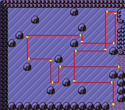
Ricochet Robots is basically the same, except you have 5 robots (4 on older versions) to bounce around. Importantly this means that you can bounce off other robots! For example in the following puzzle you can see that in move 3 the yellow bot uses the red bot to stop its movement.

The Solver
I love the game, but you quickly wonder how good you really are. That puzzle requires 22 moves? Surely there is a better option! I talked about writing a solver with some coworkers over lunch and before you know it three of us were inspired to try our hand. We sketched out an interchange format and we were off to the races.
Scale of the Problem
From the start it is clear that brute-force fuzzing is only going to work for the simplest of problems. There are 5 robots and each robot can move in up to 4 directions. This makes the worst-case complexity O((5×4)n)\O{\left(5 \times 4\right)^n}. For a pretty modest 10-move solution that is 1e131e^{13}possible board states. If you spent a nanosecond on each solution that would take almost 3h. Using a conservative estimate of 2 available moves per robot (as they tend to be near walls a lot of the time) that goes down to 10s but 10 moves isn’t particularly long and a nanosecond per state is quite short. Even with 2 moves per bot and 1 ns per move that is three thousand years for a 20 move solution (which is uncommon but possible). The longest puzzle I have seen is 25 moves and would take 300 million years.
So we are going to need to do something much more clever if we want to solve hard puzzles. We’ll get back to that shortly.
Visited State Caching
One of the most fundamental optimizations is caching visited states. This greatly reduces the search space because for a huge number of cases the order in which you move robots doesn’t matter. For example in the following scenario does it matter if the red robot moved before the blue? No, the result is the same either way.

Fundamentally the state of the game is broken down to the board (walls, mirrors and the target) as well as the robot positions. The board state doesn’t change in a particular puzzle so all that we need to save is the robot positions. The board is 16 by 16, so we have 256 positions per robot which can conveniently be stored in a single byte. The five robot-position bytes can then be stored in a mapping (at first I used a hash map but eventually switched to a more exotic trie-like structure) without using too much memory.
This caching saves a ton of work. Most possible moves are independent of other robots, so a sequence of two moves likely results the same board state as making those moves in the opposite order. Removing the order of these independent moves from the search space cuts it down to a small fraction of what the full set of possible moves would be.
On an early version of the solver this brings the solve time for a 10 move puzzle down from 202 s and almost 100 GiB of memory to 105 ms and 10 MiB of memory. On the latest solver a 12 move puzzle goes from 217 s and 50 GiB of memory to 79 ms and 30 MiB of memory. (Larger puzzles just become infeasible) It is unsurprising that this is so effective. Duplicate states are common and both of these solvers have to store a list of visited states. So if a state is seen even twice the memory usage breaks even, and every state past that is pure profit. Runtime is harder to estimate, but these lookups are fairly inexpensive and given the exponential growth that is avoided it pays off very quickly.
Search Algorithm Search
Breadth-First Search
The first step was to pick an algorithm. At first I thought I could just use breadth-first search. Despite the high possible fanout I assumed that most states would be redundant, and it would give the shortest solution first.
This resulted in a decent solver. It can solve a 17 move puzzle in 1min 52s. Puzzles that require 17 moves or more are very rare, so this makes the solver usable for general play.
Depth-First Search
Next I experimented with an iterative depth-first solver. While it was slower than the breadth-first solver it was still useful because it used far less memory. This allowed it to solve more puzzles when compiled to WebAssembly without hitting the browser-imposed memory limit or the fundamental memory limit of 32-bit WASM. So I added it as an alternative option in the web interface. Generally I would try the breadth-first option first, but if that ran out of memory I would give this solver a try, and it did occasionally find a solution for these harder problems after locking up the browser for an extended period.
The Depth-First Search solver could solve the same 17 move puzzle in 5min 24s.
I also doubled-down on the depth-first solver memory use by removing visited state caching. This meant that it used more or less a constant amount of memory, allowing it to solve any puzzle …eventually… Unfortunately it was unbearably slow for any puzzle in which memory usage was a problem to begin with.
A*
This is where things really took a step up. Breadth-first and depth-first search are quite simple algorithms and search in a mostly random manor. A* is a variant of breath-first search that searches the most likely options first. I’m not going to give a full explanation of A* here but the basic concept is that while breath-first search is constantly taking another step on the shortest path A* takes a step on the path that has the shortest possible solution. This is done by taking the current path length and then adding an estimate of how many more moves are required to reach the target. The most important thing is that this estimate can’t be too high. That is if we estimate 4 moves than it must be impossible to reach the target in less than 4 moves. We can then sort our exploration based on this estimated total path length.
It may seem hard to estimate. How can we know the length of a path that we haven’t found yet? But it turns out that this estimate is incredibly helpful even if it is quite conservative. For Ricochet Robots one possible estimate is what is the minimum number of turns that are needed if we can stop wherever is most convenient and if we can pass though other robots if required. Basically we assume that all the other robots are right where we need them and take the shortest path.
Here is an example estimate for the red robot. We can see that this path is clearly not possible in 4 moves, as it stops before hitting a wall twice then proceeds directly through another robot. However it will serve as a lower bound.

One nice feature of this estimate is that it only depends on static puzzle sate and the position of the target robot. So we can simply precompute the estimate for every cell, then scoring board positions is just a table lookup based on the location of the target robot.

With that table computed we can quickly see what the minimum score for a possible solution is, even though we haven’t completed the search. If we have already taken 3 moves and the red robot is on a 4 cell we know that a complete solution will take at least 7 moves.
Colours and Estimates
In general you only need to check the robot that is the same colour as the target against the estimate as it is the only one that needs to move to finish the puzzle. However the wild target is different, any robot can be moved there to complete the puzzle. For wild targets you need to check every robot and see the minimum of the minimum move scores. However if gets even more complicated when there are mirrors on the board. Mirrors mean that different colour robots have different movement options. A mirror could block a robot and raise its minimum or it could give the robot a “free” turn to lower it. So for puzzles with mirrors and a wild target you need to compute a different estimate map for every robot.
Right now I actually always calculate one estimate map per robot. They are very cheap to compute as they only need to be done once per board. For coloured targets only one map is ever accessed so the overhead is likely negligible. It wastes 1 kiB of stack space but in order to save that we would need to dynamically allocate so that is likely a good tradeoff. For colourless targets on boards without mirrors there is likely a small performance loss because all of these mappings will be used even though they are the same. Cache hit rate could be improved by using one map for all robots on boards without mirrors.
Board Storage
The next factor was how to represent the puzzle in memory. The solver will continuously access the game board so it was important to be fast to access. Size was also important as the smaller this data is the more likely it is to be in the processor’s cache.
The original schema was pretty straight-forward.
struct Game {
    horizontal_walls: [u16; 16],
    vertical_walls: [u16; 16],
    target: Target {
        color: Option<Robot> /* 1 byte */,
        position: Position /* 1 byte */,
    },
    mirrors: [[Mirror /* 1 byte */; 16]; 16],
    robots: [Position /* 1 byte */; 5],
}
This is pretty close to optimal space usage for arbitrary boards. There are only a few inefficacies:
- Mirrors use 1 byte each. There are only angles× colors+ absent=2×5+1=11\u{angles} \times \u{colors} + \u{absent} = 2 \times 5 + 1 = 11possibilities which rounds up to 4 bits. So 4 wasted bits per mirror, 128 bytes in total.
- The target color only needs 6 options which rounds up to 4 bits. 4 wasted bits.
- There are only really 15 possible walls per row and column, the first and last wall are always present. 4 wasted bytes.
However performance isn’t great. Checking if a robot can move forward a square requires checking:
- Is there a wall in the way. (1 bit lookup by index)
- Is there a mirror in the target location? (1 byte lookup by index)
- Is there a robot in the target location? (search 5 bytes)
It sounds small but moving the robot does these checks for each cell moved and moving is the most frequent operation in the game.
Obstacle Bitmap
The first optimization was to add a fast lookup for obstacles.
obstacles: [u16; 16],
One bit per cell is a small price to pay. Every robot and mirror was set in this table. Now in most cases we could get a negative result for both robot and mirror collisions quickly. This made a nice improvement to performance, but would eventually be superseded.
One oversight was that disambiguation between a robot and a mirror was done by checking the mirror map. If there was no mirror the collision must have been a robot. This resulted in relatively frequent access to the mirror map even if there were no mirror there. This was done to avoid searching the robot list but was likely too high a price to pay. Especially for puzzles with no mirrors.
Per-Direction Obstacle Map
A failed optimization attempt was to merge walls into the obstacle map. The first issue is that walls are “between” cells. So they didn’t fit naturally into the bitmap. If a cell was blocked depended on what direction the robot was moving from.
This resulted in an attempt to build an obstacle bitmap for each direction. This way a 0 in the bit for a cell was a guaranteed free cell. It also means that we could use bit counting counting instructions to tell not just if a cell was free quickly, but how many cells are free in that direction. So instead of moving and checking one cell at a time we could directly identify the target cell (or the mirror that we would bounce on). Surely this change from iteration to direct jumping would improve performance.
fn move_distance(lane: u16, pos: i) -> u8 {
    (lane >> pos).trailing_zeros() as u8
}
Unfortunately this didn’t end up improving performance. I may want to revisit in the future as it seems like it should work, but benchmarks showed ~10% slowdown. It turns out that computers can run simple loops very fast! While I don’t have a detailed analysis on the slowdown I have a few ideas:
- Normalizing the
posto be relative to the direction required some branching. (Could likely be optimized.) - Still looked into the
mirrorsmap on a hit. - Moving a robot required updating 4 obstacle maps. Updating these maps also required checking a reference wall map to determine if removing a robot cleared an obstacle (as moving a robot behind a wall should not clear the obstacle bit). So the regular wall maps were still being used during solving.
Cell-Oriented Map
At this point I tried to grow my obstacle map to encompass everything required for moving through a cell. This means I would pack the following into one byte:
- All 4 walls.
- If a robot is present.
- Full information about a mirror.
Packing this into 8 bits isn’t obvious, but it is possible without any hackery.
4 walls are simply one bit each. Without assuming anything about the board we have to assume that every combination is possible. This does duplicate every wall (as the east wall of this cell is the west wall of the next cell) but we wanted to have all the info we needed in one place.
The next 4 bits pack in robot presence and mirror info. Importantly a robot can’t be on a mirror cell. So we use this exclusivity to pack the data into one nibble (values 0-15). We reserve one value (15) for an empty cell, and one value (14) for a cell with a robot in it. The remaining 14 values are used for mirror information. A mirror is defined by the lean (top-left to bottom-right or top-right to bottom-left) and robot colour. The lean is one bit, so we are left with 7 options for robot colour. Luckily we only have 5 robots (the original game has no black mirrors, but we support it) so it fits with a few values to spare.
enum Contents { Empty, Robot, Mirror(Mirror) }

fn parse_cell(cell: u8) -> (Walls, Contents) {
    let walls = Walls::from_u4(cell & 0x0F);
    let contents = match cell >> 4 {
        15 => Contents::Empty,
        14 => Contents::Robot,
        mirror => {
            let left_leaning = mirror & 0x01 != 0;
            let color = Robot::try_from(mirror >> 1).uwnrap();
            Contents::Mirror(Mirror::new(left_leaning, color))
        }
    };
    (walls, contents)
}
This was surprisingly effective, resulting in a 15% performance improvement. With this we could completely remove the previous wall representation and mirror map from the solver. This reduced our core data to only 263 bytes:
struct Game {
    board: [[u8; 16]; 16], // Contains walls, mirrors and obstacle map.
    target: Target,
    robots: [Position; 5],
}
Improved A* Estimate
The previous estimate was very cheap to calculate, but not particularly accurate. To make it more accurate a penalty was added if the minimum path isn’t possible. If the minimum path requires mid-air turns or passing through a robot the minimum solution is clearly unobtainable. At least one extra move will be required to move a blocker into or out of your path. I couldn’t find an easy way to make the penalty more than one, it seems like doing so would be essentially solving the optimal path again.
So this path-check is much more expensive and can only improve the estimate by a single point, is it actually an improvement? Absolutely! This change made some complex puzzles solve in half the time! This serves as a great reminder than even minor algorithmic improvements can trounce tons of micro-optimizations.
Making this estimate even better is a clear area for future optimizations. I think the current estimate is pretty good but even minor improvements will provide great value.
Robot Sorting
In Michael Fogleman’s talk about his solver uses a technique of sorting all of the robots. This makes the Visited State Caching more effective by making equivalent states identical. There is one important complication though, Michael is solving an earlier edition of the game without mirrors. I actually had a simplified sorting system for the depth-first search solver to prefer moving the target robot, but it was removed when mirror support was added. Without mirrors robots are identical (other than the robot that matches a coloured target). With mirrors each robot is unique as the possible moves it can make depend on its colour. I decided to try sorting anyway since many puzzles don’t have mirrors (or only have a couple).
The implementation is quite simple. I “pin” any robot that is the same colour as the target or any mirror. All of the unpinned robots are then sorted before being put into the visited state cache. Some care then needs to be taken to “unsort” the robots when generating the solution.
To make this a little more efficient I sort the pinned robots to the start of the robot list before starting solving. The target and mirror colours are then updated to match the changes. This is done once per game, then while solving I just self.robots[self.pinned_robot_count()..].sort() to sort the unpinned robots.
Robot sorting had some big improvements but it depended a lot on how many robots were pinned.
- Games with a wild target and no mirrors saw 50% improvement. (No robots pinned)
- Games without mirrors saw 30% improvement. (One robot pinned)
- Games with all robots pinned saw no significant slowdown.
Since no games were slowed down it made sense to just enable this for all games.
Summary
After these optimizations I have created the fastest Ricochet Robots solver that I am aware of. You can try it online or browse the source code
To summarize my approach:
- Cache visited states, there is a huge amount of redundancy.
- A* search with an estimate function based on being able to turn at any point.
- One penalty move if the route isn’t possible.
- Sort robots to erase any insignificant colours.
- Minimize working set size and try to keep cache locality.
That’s all for now. If you haven’t played yet you should, it is my favourite game. (Although I think it is out of print so it may be hard to find.) If you do, try my solver on some of the harder puzzles, it can help you learn new techniques.


Top comments (0)