
This is the latest in my series of screencasts demonstrating how to use the tidymodels packages, from starting out with first modeling steps to tuning more complex models. Today’s screencast walks through how to tune, fit, and predict from decision tree models, using this week’s #TidyTuesday dataset on Canadian wind turbines. 🇨🇦
Here is the code I used in the video, for those who prefer reading instead of or in addition to video.
Explore data
Our modeling goal is to predict the capacity of wind turbines in Canada based on other characteristics of the turbines from this week’s #TidyTuesday dataset. Simon Couch outlined this week how to use stacks for ensembling with this dataset, but here let’s take a more straightforward approach.
Let’s start by reading in the data.
library(tidyverse)

turbines <- read_csv("https://raw.githubusercontent.com/rfordatascience/tidytuesday/master/data/2020/2020-10-27/wind-turbine.csv")
turbines


## # A tibble: 6,698 x 15
## objectid province_territ… project_name total_project_c… turbine_identif…
## <dbl> <chr> <chr> <dbl> <chr>
## 1 1 Alberta Optimist Wi… 0.9 OWE1
## 2 2 Alberta Castle Rive… 44 CRW1
## 3 3 Alberta Waterton Wi… 3.78 WWT1
## 4 4 Alberta Waterton Wi… 3.78 WWT2
## 5 5 Alberta Waterton Wi… 3.78 WWT3
## 6 6 Alberta Waterton Wi… 3.78 WWT4
## 7 7 Alberta Cowley North 19.5 CON1
## 8 8 Alberta Cowley North 19.5 CON2
## 9 9 Alberta Cowley North 19.5 CON3
## 10 10 Alberta Cowley North 19.5 CON4
## # … with 6,688 more rows, and 10 more variables:
## # turbine_number_in_project <chr>, turbine_rated_capacity_k_w <dbl>,
## # rotor_diameter_m <dbl>, hub_height_m <dbl>, manufacturer <chr>,
## # model <chr>, commissioning_date <chr>, latitude <dbl>, longitude <dbl>,
## # notes <chr>
Let’s do a bit of data cleaning and preparation.
turbines_df <- turbines %>%
  transmute(
    turbine_capacity = turbine_rated_capacity_k_w,
    rotor_diameter_m,
    hub_height_m,
    commissioning_date = parse_number(commissioning_date),
    province_territory = fct_lump_n(province_territory, 10),
    model = fct_lump_n(model, 10)
  ) %>%
  filter(!is.na(turbine_capacity)) %>%
  mutate_if(is.character, factor)
How is the capacity related to other characteristics like the year of commissioning or size of the turbines?
turbines_df %>%
  select(turbine_capacity:commissioning_date) %>%
  pivot_longer(rotor_diameter_m:commissioning_date) %>%
  ggplot(aes(turbine_capacity, value)) +
  geom_hex(bins = 15, alpha = 0.8) +
  geom_smooth(method = "lm") +
  facet_wrap(~name, scales = "free_y") +
  labs(y = NULL) +
  scale_fill_gradient(high = "cyan3")

These relationships are the kind that we want to use in modeling, whether that’s the modeling stacking Simon demonstrated or the single model we’ll use here.
Build a model
We can start by loading the tidymodels metapackage, splitting our data into training and testing sets, and creating cross-validation samples.
library(tidymodels)

set.seed(123)
wind_split <- initial_split(turbines_df, strata = turbine_capacity)
wind_train <- training(wind_split)
wind_test <- testing(wind_split)

set.seed(234)
wind_folds <- vfold_cv(wind_train, strata = turbine_capacity)
wind_folds


## # 10-fold cross-validation using stratification
## # A tibble: 10 x 2
## splits id
## <list> <chr>
## 1 <split [4.4K/488]> Fold01
## 2 <split [4.4K/487]> Fold02
## 3 <split [4.4K/486]> Fold03
## 4 <split [4.4K/486]> Fold04
## 5 <split [4.4K/486]> Fold05
## 6 <split [4.4K/486]> Fold06
## 7 <split [4.4K/486]> Fold07
## 8 <split [4.4K/486]> Fold08
## 9 <split [4.4K/485]> Fold09
## 10 <split [4.4K/484]> Fold10
Next, let’s create a tunable decision tree model specification.
tree_spec <- decision_tree(
  cost_complexity = tune(),
  tree_depth = tune(),
  min_n = tune()
) %>%
  set_engine("rpart") %>%
  set_mode("regression")

tree_spec


## Decision Tree Model Specification (regression)
##
## Main Arguments:
## cost_complexity = tune()
## tree_depth = tune()
## min_n = tune()
##
## Computational engine: rpart
We need a set of possible parameter values to try out for the decision tree.
tree_grid <- grid_regular(cost_complexity(), tree_depth(), min_n(), levels = 4)

tree_grid


## # A tibble: 64 x 3
## cost_complexity tree_depth min_n
## <dbl> <int> <int>
## 1 0.0000000001 1 2
## 2 0.0000001 1 2
## 3 0.0001 1 2
## 4 0.1 1 2
## 5 0.0000000001 5 2
## 6 0.0000001 5 2
## 7 0.0001 5 2
## 8 0.1 5 2
## 9 0.0000000001 10 2
## 10 0.0000001 10 2
## # … with 54 more rows
Now, let’s try out all the possible parameter values on all our resampled datasets. Let’s use some non-default metrics, while we’re at it.
doParallel::registerDoParallel()

set.seed(345)
tree_rs <- tune_grid(
  tree_spec,
  turbine_capacity ~ .,
  resamples = wind_folds,
  grid = tree_grid,
  metrics = metric_set(rmse, rsq, mae, mape)
)

tree_rs


## # Tuning results
## # 10-fold cross-validation using stratification
## # A tibble: 10 x 4
## splits id .metrics .notes
## <list> <chr> <list> <list>
## 1 <split [4.4K/488]> Fold01 <tibble [256 × 7]> <tibble [0 × 1]>
## 2 <split [4.4K/487]> Fold02 <tibble [256 × 7]> <tibble [0 × 1]>
## 3 <split [4.4K/486]> Fold03 <tibble [256 × 7]> <tibble [0 × 1]>
## 4 <split [4.4K/486]> Fold04 <tibble [256 × 7]> <tibble [0 × 1]>
## 5 <split [4.4K/486]> Fold05 <tibble [256 × 7]> <tibble [0 × 1]>
## 6 <split [4.4K/486]> Fold06 <tibble [256 × 7]> <tibble [0 × 1]>
## 7 <split [4.4K/486]> Fold07 <tibble [256 × 7]> <tibble [0 × 1]>
## 8 <split [4.4K/486]> Fold08 <tibble [256 × 7]> <tibble [0 × 1]>
## 9 <split [4.4K/485]> Fold09 <tibble [256 × 7]> <tibble [0 × 1]>
## 10 <split [4.4K/484]> Fold10 <tibble [256 × 7]> <tibble [0 × 1]>
Notice that we aren’t tuning a workflow() here, as I have often shown how to do. Instead we are tuning the model specification (accompanied by a formula preprocessor); this is so we can use the bare model in some model evaluation activities.
Evaluate model
Now let’s check out how we did. We can collect or visualize the metrics.
collect_metrics(tree_rs)


## # A tibble: 256 x 9
## cost_complexity tree_depth min_n .metric .estimator mean n std_err
## <dbl> <int> <int> <chr> <chr> <dbl> <int> <dbl>
## 1 0.0000000001 1 2 mae standard 386. 10 1.50
## 2 0.0000000001 1 2 mape standard 27.7 10 1.30
## 3 0.0000000001 1 2 rmse standard 508. 10 1.44
## 4 0.0000000001 1 2 rsq standard 0.303 10 0.0134
## 5 0.0000001 1 2 mae standard 386. 10 1.50
## 6 0.0000001 1 2 mape standard 27.7 10 1.30
## 7 0.0000001 1 2 rmse standard 508. 10 1.44
## 8 0.0000001 1 2 rsq standard 0.303 10 0.0134
## 9 0.0001 1 2 mae standard 386. 10 1.50
## 10 0.0001 1 2 mape standard 27.7 10 1.30
## # … with 246 more rows, and 1 more variable: .config <chr>


autoplot(tree_rs) + theme_light(base_family = "IBMPlexSans")
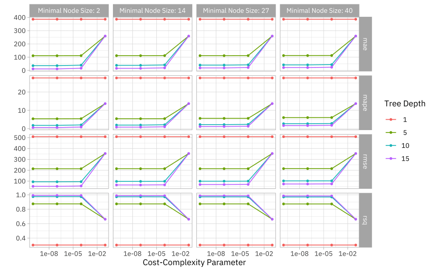
Looks like this data needs a fairly complex tree!
We can examine or select the best sets of parameter options, chosen by whichever metric we want.
show_best(tree_rs, "mape")


## # A tibble: 5 x 9
## cost_complexity tree_depth min_n .metric .estimator mean n std_err
## <dbl> <int> <int> <chr> <chr> <dbl> <int> <dbl>
## 1 0.0000000001 15 2 mape standard 0.564 10 0.0592
## 2 0.0000001 15 2 mape standard 0.564 10 0.0591
## 3 0.0000000001 15 14 mape standard 0.823 10 0.0547
## 4 0.0000001 15 14 mape standard 0.823 10 0.0547
## 5 0.0001 15 2 mape standard 0.885 10 0.0705
## # … with 1 more variable: .config <chr>


select_best(tree_rs, "rmse")


## # A tibble: 1 x 4
## cost_complexity tree_depth min_n .config
## <dbl> <int> <int> <chr>
## 1 0.0000000001 15 2 Preprocessor1_Model13
Next, let’s use one of these “best” sets of parameters to update and finalize our model.
final_tree <- finalize_model(tree_spec, select_best(tree_rs, "rmse"))

final_tree


## Decision Tree Model Specification (regression)
##
## Main Arguments:
## cost_complexity = 1e-10
## tree_depth = 15
## min_n = 2
##
## Computational engine: rpart
This model final_tree is updated and finalized (no longer tunable) but it is not fit. It has all its hyperparameters set but it has not been fit to any data. We have a couple of options for how to fit this model. We can either fit final_tree to training data using fit() or to the testing/training split using last_fit(), which will give us some other results along with the fitted output.
final_fit <- fit(final_tree, turbine_capacity ~ ., wind_train)
final_rs <- last_fit(final_tree, turbine_capacity ~ ., wind_split)
We can predict from either one of these objects.
predict(final_fit, wind_train[144,])


## # A tibble: 1 x 1
## .pred
## <dbl>
## 1 1800


predict(final_rs$.workflow[[1]], wind_train[144,])


## # A tibble: 1 x 1
## .pred
## <dbl>
## 1 1800
What are the most important variables in this decision tree for predicting turbine capacity?
library(vip)

final_fit %>%
  vip(geom = "col", aesthetics = list(fill = "midnightblue", alpha = 0.8)) +
  scale_y_continuous(expand = c(0, 0))

I really like the parttree package for visualization decision tree results. It only works for models with one or two predictors, so we’ll have to fit an example model that isn’t quite the same as our full model. It can still help us understand how this decision tree is working, but keep in mind that it is not the same as our full model with more predictors.
library(parttree)

ex_fit <- fit(
  final_tree,
  turbine_capacity ~ rotor_diameter_m + commissioning_date,
  wind_train
)

wind_train %>%
  ggplot(aes(rotor_diameter_m, commissioning_date)) +
  geom_parttree(data = ex_fit, aes(fill = turbine_capacity), alpha = 0.3) +
  geom_jitter(alpha = 0.7, width = 1, height = 0.5, aes(color = turbine_capacity)) +
  scale_colour_viridis_c(aesthetics = c("color", "fill"))

Finally, let’s turn to the testing data! These results are stored in final_rs, along with the fitted output there. We can see both metrics on the testing data and predictions.
collect_metrics(final_rs)


## # A tibble: 2 x 4
## .metric .estimator .estimate .config
## <chr> <chr> <dbl> <chr>
## 1 rmse standard 73.6 Preprocessor1_Model1
## 2 rsq standard 0.985 Preprocessor1_Model1


final_rs %>%
  collect_predictions() %>%
  ggplot(aes(turbine_capacity, .pred)) +
  geom_abline(slope = 1, lty = 2, color = "gray50", alpha = 0.5) +
  geom_point(alpha = 0.6, color = "midnightblue") +
  coord_fixed()


Top comments (0)