
Lately I’ve been publishing screencasts demonstrating how to use the tidymodels framework, from starting out with first modeling steps to tuning more complex models. Today’s screencast walks through how to tune and choose hyperparameters using this week’s #TidyTuesday dataset on NCAA women’s basketball tournaments. ⛹️♀️
Here is the code I used in the video, for those who prefer reading instead of or in addition to video.
Explore the data
Our modeling goal is to estimate the relationship of expected tournament wins by seed from this week’s #TidyTuesday dataset. This is similar to the “average” column in the FiveThirtyEight table in this article. This was what I was most interested in when I saw this data, but I was pretty confused about what was going on this table at first! Many thanks to Tom Mock for helping out my understanding.
Let’s start by reading in the data.
library(tidyverse)
tournament <- read_csv("https://raw.githubusercontent.com/rfordatascience/tidytuesday/master/data/2020/2020-10-06/tournament.csv")

tournament


## # A tibble: 2,092 x 19
## year school seed conference conf_w conf_l conf_percent conf_place reg_w
## <dbl> <chr> <dbl> <chr> <dbl> <dbl> <dbl> <chr> <dbl>
## 1 1982 Arizo… 4 Western C… NA NA NA - 23
## 2 1982 Auburn 7 Southeast… NA NA NA - 24
## 3 1982 Cheyn… 2 Independe… NA NA NA - 24
## 4 1982 Clems… 5 Atlantic … 6 3 66.7 4th 20
## 5 1982 Drake 4 Missouri … NA NA NA - 26
## 6 1982 East … 6 Independe… NA NA NA - 19
## 7 1982 Georg… 5 Southeast… NA NA NA - 21
## 8 1982 Howard 8 Mid-Easte… NA NA NA - 14
## 9 1982 Illin… 7 Big Ten NA NA NA - 21
## 10 1982 Jacks… 7 Southwest… NA NA NA - 28
## # … with 2,082 more rows, and 10 more variables: reg_l <dbl>,
## # reg_percent <dbl>, how_qual <chr>, x1st_game_at_home <chr>,
## # tourney_w <dbl>, tourney_l <dbl>, tourney_finish <chr>, full_w <dbl>,
## # full_l <dbl>, full_percent <dbl>
We can look at the mean wins by seed.
tournament %>%
  group_by(seed) %>%
  summarise(exp_wins = mean(tourney_w, na.rm = TRUE)) %>%
  ggplot(aes(seed, exp_wins)) +
  geom_point(alpha = 0.8, size = 3) +
  labs(y = "tournament wins (mean)")

Let’s visualize all the tournament results, not just the averages.
tournament %>%
  ggplot(aes(seed, tourney_w)) +
  geom_bin2d(binwidth = c(1, 1), alpha = 0.8) +
  scale_fill_gradient(low = "gray85", high = "midnightblue") +
  labs(fill = "number of\nteams", y = "tournament wins")
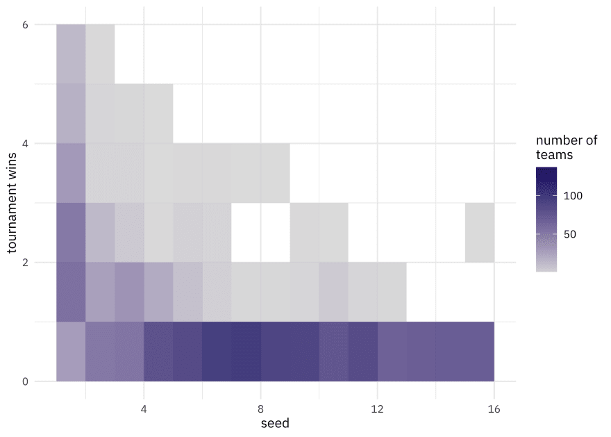
We have a lot of options to deal with data like this (curvy, integers, all greater than zero) but one straightforward option are splines. Splines aren’t perfect for this because they aren’t constrained to stay greater than zero or to always decrease, but they work pretty well and can be used in lots of situations. We have to choose the degrees of freedom for the splines.
library(splines)

plot_smoother <- function(deg_free) {
  p <- ggplot(tournament, aes(seed, tourney_w)) +
    geom_bin2d(binwidth = c(1, 1), alpha = 0.8) +
    scale_fill_gradient(low = "gray85", high = "midnightblue") +
    geom_smooth(
      method = lm, se = FALSE, color = "black",
      formula = y ~ ns(x, df = deg_free)
    ) +
    labs(
      fill = "number of\nteams", y = "tournament wins",
      title = paste(deg_free, "spline terms")
    )

  print(p)
}

walk(c(2, 4, 6, 8, 10, 15), plot_smoother)

As the number of degrees of freedom goes up, the curves get more wiggly. This would allow the model to fit a more complex relationship, perhaps too much so give our data. We can tune this hyperparameter to find the best value.
Build a model
We can start by loading the tidymodels metapackage, and splitting our data into training and testing sets.
library(tidymodels)

set.seed(123)
tourney_split <- tournament %>%
  filter(!is.na(seed)) %>%
  initial_split(strata = seed)

tourney_train <- training(tourney_split)
tourney_test <- testing(tourney_split)
We are going to use resampling to evaluate model performance, so let’s get those resampled sets ready.
set.seed(234)
tourney_folds <- bootstraps(tourney_train)
tourney_folds


## # Bootstrap sampling
## # A tibble: 25 x 2
## splits id
## <list> <chr>
## 1 <split [1.6K/545]> Bootstrap01
## 2 <split [1.6K/587]> Bootstrap02
## 3 <split [1.6K/597]> Bootstrap03
## 4 <split [1.6K/581]> Bootstrap04
## 5 <split [1.6K/581]> Bootstrap05
## 6 <split [1.6K/597]> Bootstrap06
## 7 <split [1.6K/570]> Bootstrap07
## 8 <split [1.6K/572]> Bootstrap08
## 9 <split [1.6K/598]> Bootstrap09
## 10 <split [1.6K/576]> Bootstrap10
## # … with 15 more rows
Next we build a recipe for data preprocessing. It only has one step!
- First, we must tell the
recipe()what our model is going to be (using a formula here) and what our training data is. - For our first and only step, we create new spline terms from the original
seedvariable. We don’t know what the best value for the degrees of freedom is, so we willtune()it. We can set anidvalue for the tuneable parameter to more easily keep track of it, if we want.
The object tourney_rec is a recipe that has not been trained on data yet, and in fact, we can’t do this because we haven’t decided on a value for deg_free.
tourney_rec <- recipe(tourney_w ~ seed, data = tourney_train) %>%
  step_ns(seed, deg_free = tune("seed_splines"))

tourney_rec


## Data Recipe
##
## Inputs:
##
## role #variables
## outcome 1
## predictor 1
##
## Operations:
##
## Natural Splines on seed
Next, let’s create a model specification for a linear regression model, and the combine the recipe and model together in a workflow.
lm_spec <- linear_reg() %>% set_engine("lm")

tourney_wf <- workflow() %>%
  add_recipe(tourney_rec) %>%
  add_model(lm_spec)

tourney_wf


## ══ Workflow ════════════════════════════════════════════════════════════════════════════════════════════
## Preprocessor: Recipe
## Model: linear_reg()
##
## ── Preprocessor ────────────────────────────────────────────────────────────────────────────────────────
## 1 Recipe Step
##
## ● step_ns()
##
## ── Model ───────────────────────────────────────────────────────────────────────────────────────────────
## Linear Regression Model Specification (regression)
##
## Computational engine: lm
This workflow is almost ready to go, but we need to decide what values to try for the splines. There are several different ways to create tuning grids, but if the grid you need is very simple, you might prefer to create it by hand.
spline_grid <- tibble(seed_splines = c(1:3, 5, 7, 10))
spline_grid


## # A tibble: 6 x 1
## seed_splines
## <dbl>
## 1 1
## 2 2
## 3 3
## 4 5
## 5 7
## 6 10
Now we can put this all together! When we use tune_grid(), we will fit each of the options in the grid to each of the resamples.
doParallel::registerDoParallel()
save_preds <- control_grid(save_pred = TRUE)

spline_rs <-
  tune_grid(
    tourney_wf,
    resamples = tourney_folds,
    grid = spline_grid,
    control = save_preds
  )

spline_rs


## # Tuning results
## # Bootstrap sampling
## # A tibble: 25 x 5
## splits id .metrics .notes .predictions
## <list> <chr> <list> <list> <list>
## 1 <split [1.6K/54… Bootstrap… <tibble [12 × … <tibble [0 × … <tibble [3,270 × …
## 2 <split [1.6K/58… Bootstrap… <tibble [12 × … <tibble [0 × … <tibble [3,522 × …
## 3 <split [1.6K/59… Bootstrap… <tibble [12 × … <tibble [0 × … <tibble [3,582 × …
## 4 <split [1.6K/58… Bootstrap… <tibble [12 × … <tibble [0 × … <tibble [3,486 × …
## 5 <split [1.6K/58… Bootstrap… <tibble [12 × … <tibble [0 × … <tibble [3,486 × …
## 6 <split [1.6K/59… Bootstrap… <tibble [12 × … <tibble [0 × … <tibble [3,582 × …
## 7 <split [1.6K/57… Bootstrap… <tibble [12 × … <tibble [0 × … <tibble [3,420 × …
## 8 <split [1.6K/57… Bootstrap… <tibble [12 × … <tibble [0 × … <tibble [3,432 × …
## 9 <split [1.6K/59… Bootstrap… <tibble [12 × … <tibble [0 × … <tibble [3,588 × …
## 10 <split [1.6K/57… Bootstrap… <tibble [12 × … <tibble [0 × … <tibble [3,456 × …
## # … with 15 more rows
We have now fit each of our candidate set of spline features to our resampled training set!
Evaluate model
Now let’s check out how we did.
collect_metrics(spline_rs)


## # A tibble: 12 x 7
## seed_splines .metric .estimator mean n std_err .config
## <dbl> <chr> <chr> <dbl> <int> <dbl> <chr>
## 1 1 rmse standard 0.982 25 0.00741 Recipe1
## 2 1 rsq standard 0.432 25 0.00372 Recipe1
## 3 2 rmse standard 0.896 25 0.00749 Recipe2
## 4 2 rsq standard 0.528 25 0.00486 Recipe2
## 5 3 rmse standard 0.871 25 0.00727 Recipe3
## 6 3 rsq standard 0.554 25 0.00518 Recipe3
## 7 5 rmse standard 0.869 25 0.00730 Recipe4
## 8 5 rsq standard 0.556 25 0.00541 Recipe4
## 9 7 rmse standard 0.868 25 0.00718 Recipe5
## 10 7 rsq standard 0.557 25 0.00537 Recipe5
## 11 10 rmse standard 0.868 25 0.00693 Recipe6
## 12 10 rsq standard 0.557 25 0.00538 Recipe6
Looks like the model got better and better as we added more degrees of freedom, which isn’t too shocking. In what way did it change?
collect_metrics(spline_rs) %>%
  ggplot(aes(seed_splines, mean, color = .metric)) +
  geom_line(size = 1.5, alpha = 0.5) +
  geom_point(size = 3) +
  facet_wrap(~.metric, ncol = 1, scales = "free_y") +
  labs(x = "degrees of freedom", y = NULL) +
  theme(legend.position = "none")
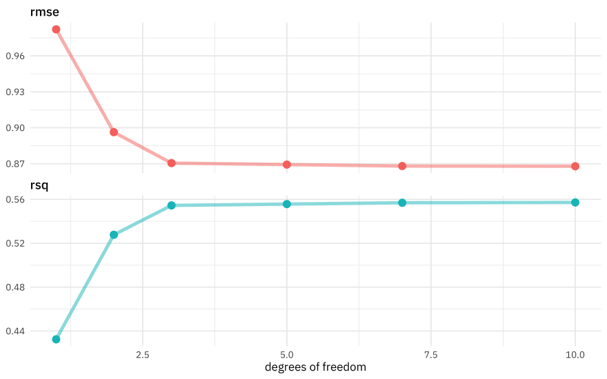
The model improved a lot as we increased the degrees of freedom at the beginning, but then continuing to add more didn’t make much difference. We could choose the numerically optimal hyperparameter with select_best() but that would choose a more wiggly, complex model than we probably want. We can choose a simpler model that performs well, within some limits around the numerically optimal result. We could choose either by percent loss in performance or within one standard error in performance.
select_by_pct_loss(spline_rs, metric = "rmse", limit = 5, seed_splines)


## # A tibble: 1 x 9
## seed_splines .metric .estimator mean n std_err .config .best .loss
## <dbl> <chr> <chr> <dbl> <int> <dbl> <chr> <dbl> <dbl>
## 1 2 rmse standard 0.896 25 0.00749 Recipe2 0.868 3.27


select_by_one_std_err(spline_rs, metric = "rmse", seed_splines)


## # A tibble: 1 x 9
## seed_splines .metric .estimator mean n std_err .config .best .bound
## <dbl> <chr> <chr> <dbl> <int> <dbl> <chr> <dbl> <dbl>
## 1 3 rmse standard 0.871 25 0.00727 Recipe3 0.868 0.875
Looks like 2 or 3 degrees of freedom is a good option. Let’s go with 3, and update our tuneable workflow with this information and then fit it to our training data.
final_wf <- finalize_workflow(tourney_wf, tibble(seed_splines = 3))
tourney_fit <- fit(final_wf, tourney_train)
tourney_fit


## ══ Workflow [trained] ══════════════════════════════════════════════════════════════════════════════════
## Preprocessor: Recipe
## Model: linear_reg()
##
## ── Preprocessor ────────────────────────────────────────────────────────────────────────────────────────
## 1 Recipe Step
##
## ● step_ns()
##
## ── Model ───────────────────────────────────────────────────────────────────────────────────────────────
##
## Call:
## stats::lm(formula = ..y ~ ., data = data)
##
## Coefficients:
## (Intercept) seed_ns_1 seed_ns_2 seed_ns_3
## 3.272 -1.855 -5.590 -1.822
We can predict from this fitted workflow. For example, we can predict on the testing data and compute model performance.
tourney_test %>%
  bind_cols(predict(tourney_fit, tourney_test)) %>%
  metrics(tourney_w, .pred)


## # A tibble: 3 x 3
## .metric .estimator .estimate
## <chr> <chr> <dbl>
## 1 rmse standard 0.877
## 2 rsq standard 0.545
## 3 mae standard 0.609
Pretty good! We can also predict on other kinds of new data. For example, let’s recreate the “average” column in the FiveThirtyEight table on expected wins.
predict(tourney_fit, new_data = tibble(seed = 1:16))


## # A tibble: 16 x 1
## .pred
## <dbl>
## 1 3.27
## 2 2.61
## 3 1.99
## 4 1.45
## 5 1.02
## 6 0.738
## 7 0.574
## 8 0.492
## 9 0.456
## 10 0.429
## 11 0.380
## 12 0.307
## 13 0.216
## 14 0.110
## 15 -0.00482
## 16 -0.125
It’s close! This isn’t a huge surprise, since we’re fitting curves to data in a straightforward way here, but it’s still good to see. You can also see why splines aren’t perfect for this task, because the prediction isn’t constrained to positive values.

Top comments (0)