Learn about log odds and empirical Bayes with cocktail 🍸 recipes

I am very pleased to announce that tidylo, a package for weighted log odds using tidy data principles, is now on CRAN! 🎉 I would like to send my warmest thanks to my collaborators Alex Hayes and Tyler Schnoebelen for their helpful contributions.

You can now install the released version of tidylo from CRAN with:

install.packages("tidylo")

A log odds ratio is a way of expressing probabilities, and we can weight a log odds ratio so that our implementation does a better job dealing with different features having different counts. In particular, we use the method outlined in Monroe, Colaresi, and Quinn (2008) for posterior log odds ratios, assuming a multinomial model with a Dirichlet prior. The default prior is estimated from the data itself , an empirical Bayesian approach, but an uninformative prior is also available.

Text analysis is a main motivator for this implementation of weighted log odds, because natural language exhibits an approximately power distribution for word counts with some words counted many times and others counted only a few times. Check out both the README and the package vignette for examples using text mining. However, this weighted log odds approach is a general one for measuring how much more likely one feature (any kind of feature, not just a word or bigram) is to be associated than another for some set or group (any kind of set, not just a document or book).

Cocktail ingredients

To demonstrate this, let’s examine this week’s #TidyTuesday dataset of cocktail recipes, focusing on the ingredients in the cocktails and the type of glasses 🍸 the cocktails are served in. This is a good fit for the weighted log odds approach because some ingredients (like vodka) are much more common than others (like tabasco sauce). Which ingredients are more likely to be used with which type of cocktail glass, using a prior estimated from the data itself? By weighting using empirical Bayes estimation, we take into account the uncertainty in our measurements and acknowledge that we are more certain when we’ve counted something a lot of times and less certain when we’ve counted something only a few times. When weighting by the prior in this way, we focus on differences that are more likely to be real, given the evidence that we have.

Let’s convert both the cocktail glass and ingredient columns to lower case (because there are some differences in capitalization across rows), and count up totals for each combination.

library(tidyverse)
library(tidylo)
library(tidytuesdayR)

tuesdata <- tt_load(2020, week = 22)
cocktails <- tuesdata$cocktails

cocktail_counts <- cocktails %>%
  mutate(
    glass = str_to_lower(glass),
    ingredient = str_to_lower(ingredient)
  ) %>%
  count(glass, ingredient, sort = TRUE)

cocktail_counts


## # A tibble: 900 x 3
## glass ingredient n
## <chr> <chr> <int>
## 1 cocktail glass gin 39
## 2 collins glass vodka 24
## 3 cocktail glass dry vermouth 19
## 4 cocktail glass lemon juice 19
## 5 cocktail glass triple sec 19
## 6 collins glass sugar 19
## 7 highball glass vodka 18
## 8 highball glass gin 16
## 9 collins glass orange juice 15
## 10 highball glass orange juice 15
## # … with 890 more rows

Now let’s use the bind_log_odds() function from the tidylo package to find the weighted log odds for each bigram. The weighted log odds computed by this function are also z-scores for the log odds; this quantity is useful for comparing frequencies across categories or sets but its relationship to an odds ratio is not straightforward after the weighting.

What are the ingredients with the highest weighted log odds for these glasses?

cocktail_log_odds <- cocktail_counts %>%
  bind_log_odds(glass, ingredient, n) 

cocktail_log_odds %>%
  filter(n > 5) %>%
  arrange(-log_odds_weighted)


## # A tibble: 83 x 4
## glass ingredient n log_odds_weighted
## <chr> <chr> <int> <dbl>
## 1 coffee mug coffee 10 8.52
## 2 coffee mug chocolate 6 8.25
## 3 coffee mug sugar 6 7.94
## 4 coffee mug milk 11 7.63
## 5 champagne flute champagne 6 7.26
## 6 whiskey sour glass powdered sugar 6 6.56
## 7 highball glass yoghurt 9 6.42
## 8 cocktail glass orange bitters 11 6.35
## 9 cocktail glass dry vermouth 19 6.32
## 10 shot glass bailey's irish cream 9 5.91
## # … with 73 more rows

We can see right away that the highest weighted log odds ingredients in the dataset are coffee, chocolate, sugar, and milk for a coffee mug. Let’s create a visualization to see the highest weighted log odds ingredients for four different types of glasses.

library(tidytext)

glasses <- c("coffee mug", "champagne flute", "old-fashioned glass", "shot glass")

cocktail_log_odds %>%
  filter(glass %in% glasses) %>%
  group_by(glass) %>%
  top_n(10) %>%
  ungroup() %>%
  mutate(ingredient = reorder_within(ingredient, log_odds_weighted, glass)) %>%
  ggplot(aes(log_odds_weighted, ingredient, fill = glass)) +
  geom_col(show.legend = FALSE) +
  facet_wrap(~glass, scales = "free_y") +
  scale_y_reordered() +
  scale_x_continuous(expand = c(0, 0)) +
  labs(y = NULL, x = "Weighted log odds (empirical Bayes)")

OH BOY, seeing all these ingredients mixed up like this makes me feel a little queasy. 🤢 These are the ingredients most likely to be used with each glass, assuming the prior estimated from the data itself. Notice also that the ingredients for the coffee mug are the most distinctive, and the ingredients for the old-fashioned glass are the least distinctive.

Perhaps we want to understand one type of glass in more detail, and examine the relationship between weighted log odds and how common an ingredient is. Let’s look at the “cocktail glass”, which you might know as a martini glass.

library(ggrepel)
cocktail_log_odds %>%
  filter(glass == "cocktail glass",
         n > 5) %>%
  ggplot(aes(n, log_odds_weighted, label = ingredient)) +
  geom_hline(yintercept = 0, color = "gray50", lty = 2, size = 1.5) +
  geom_point(alpha = 0.8, color = "midnightblue") +
  geom_text_repel(family = "IBMPlexSans") +
  scale_x_log10() +
  labs(x = "Number of cocktails in dataset",
       y = "Weighted log odds (empirical Bayes)",
       title = "What ingredients are most specific to a cocktail/martini glass?",
       subtitle = "Sweet & dry vermouth are among the high log odds ingredients\nGin is both very common and likely to be used with a cocktail glass")

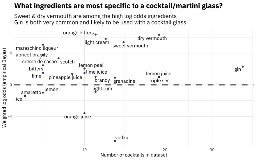
Vodka is common, but it is used among so many different kinds of glasses that is does not have a high weighted log odds for a cocktail/martini glass.

Weighty matters

By default, the prior in tidylo is estimated from the data itself as shown with the cocktail ingredients, an empirical Bayes approach, but an uninformative prior is also available. To demonstrate this, let’s look at everybody’s favorite data about cars. 🚗 What do we know about the relationship between number of gears and engine shape vs?

gear_counts <- mtcars %>%
  count(vs, gear)

gear_counts


## vs gear n
## 1 0 3 12
## 2 0 4 2
## 3 0 5 4
## 4 1 3 3
## 5 1 4 10
## 6 1 5 1

Now we can use bind_log_odds() to find the weighted log odds for each number of gears and engine shape. First, let’s use the default empirical Bayes prior. It regularizes the values.

regularized <- gear_counts %>%
  bind_log_odds(vs, gear, n)

regularized


## vs gear n log_odds_weighted
## 1 0 3 12 1.1728347
## 2 0 4 2 -1.3767516
## 3 0 5 4 0.4033125
## 4 1 3 3 -1.1354777
## 5 1 4 10 1.5661168
## 6 1 5 1 -0.4362340

For engine shape vs = 0, having three gears has the highest weighted log odds while for engine shape vs = 1, having four gears has the highest weighted log odds. This dataset is small enough that you can look at the count data and see how this is working.

Now, let’s use the uninformative prior, and compare to the unweighted log odds. These log odds will be farther from zero than the regularized estimates.

unregularized <- gear_counts %>%
  bind_log_odds(vs, gear, n, uninformative = TRUE, unweighted = TRUE)

unregularized


## vs gear n log_odds log_odds_weighted
## 1 0 3 12 0.6968169 1.8912729
## 2 0 4 2 -1.2527630 -1.9691060
## 3 0 5 4 0.3249262 0.5549172
## 4 1 3 3 -0.9673459 -1.7407107
## 5 1 4 10 1.1451323 2.8421436
## 6 1 5 1 -0.5268260 -0.6570674

Most importantly, you can notice that this approach is useful both for text data, for our example of cocktail ingredients 🥃, but also more generally whenever you have counts in some kind of groups or sets and you want to find what feature is more likely to come from a group, compared to the other groups.