This week’s #TidyTuesday datasets reflect on Juneteenth, the date when the law abolishing slavery in the United States was finally enforced throughout the American South, and specifically Texas. My own education as a white woman in the United States has been gravely lacking in the history of enslaved people, their experiences, and their impact and legacy; I’m glad to spend some time in this screencast understanding more about the forced transport of African people using the Slave Voyages African Names database.
You can find my other screencasts demonstrating how to use the tidymodels framework as well, if you are interested.
Here is the code I used in the video, for those who prefer reading instead of or in addition to video.
Explore the data
Our modeling goal is to estimate whether some characteristics of the people trafficked by enslavers changed over the last several decades of the trans-Atlantic slave trade. Missing data can be a challenge with historical data, so we’ll use imputation.
Let’s read in the data on African names and use skimr to see what’s there.
african_names <- readr::read_csv("https://raw.githubusercontent.com/rfordatascience/tidytuesday/master/data/2020/2020-06-16/african_names.csv")

skimr::skim(african_names)


## ── Data Summary ────────────────────────
## Values
## Name african_names
## Number of rows 91490
## Number of columns 11
## _______________________
## Column type frequency:
## character 6
## numeric 5
## ________________________
## Group variables None
##
## ── Variable type: character ────────────────────────────────────────────────────
## skim_variable n_missing complete_rate min max empty n_unique whitespace
## 1 name 0 1 2 24 0 62330 0
## 2 gender 12878 0.859 3 5 0 4 0
## 3 ship_name 1 1.00 2 59 0 443 0
## 4 port_disembark 0 1 6 19 0 5 0
## 5 port_embark 1126 0.988 4 31 0 59 0
## 6 country_origin 79404 0.132 3 31 0 563 0
##
## ── Variable type: numeric ──────────────────────────────────────────────────────
## skim_variable n_missing complete_rate mean sd p0 p25 p50
## 1 id 0 1 62122. 51305. 1 22935. 45822.
## 2 voyage_id 0 1 17698. 82017. 557 2443 2871
## 3 age 1126 0.988 18.9 8.60 0.5 11 20
## 4 height 4820 0.947 58.6 6.84 0 54 60
## 5 year_arrival 0 1 1831. 9.52 1808 1826 1832
## p75 p100 hist
## 1 101264. 199932 ▇▆▃▁▂
## 2 3601 500082 ▇▁▁▁▁
## 3 26 77 ▆▇▁▁▁
## 4 64 85 ▁▁▂▇▁
## 5 1837 1862 ▂▆▇▃▁
There is data missing in both the gender and age variables, two I am interested in.
This is a dataset of individual people who were liberated from slave ships. Where did the people in this dataset leave their ships?
african_names %>%
  count(port_disembark, sort = TRUE) %>%
  kable()
| port_disembark | n |
|---|---|
| Freetown | 81009 |
| Havana | 10058 |
| Bahamas unspecified | 183 |
| Kingston, Jamaica | 144 |
| St. Helena | 96 |
Most of the freed captives in this database were liberated in either Freetown, Sierra Leone (so on the eastern side of the Atlantic) or Havana, Cuba (on the western side). Both cities had tribunals/courts to judge ships seized by anti-slaving patrols after European countries outlawed or restricted slavery.
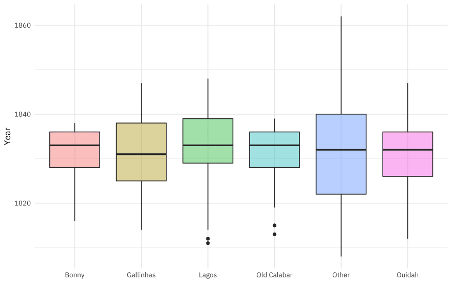
Where did these people start their forced journeys?
african_names %>%
  add_count(port_embark) %>%
  mutate(port_embark = case_when(
    n < 4000 ~ "Other",
    TRUE ~ port_embark
  )) %>%
  ggplot(aes(port_embark, year_arrival, fill = port_embark)) +
  geom_boxplot(alpha = 0.4, show.legend = FALSE) +
  labs(x = NULL, y = "Year")
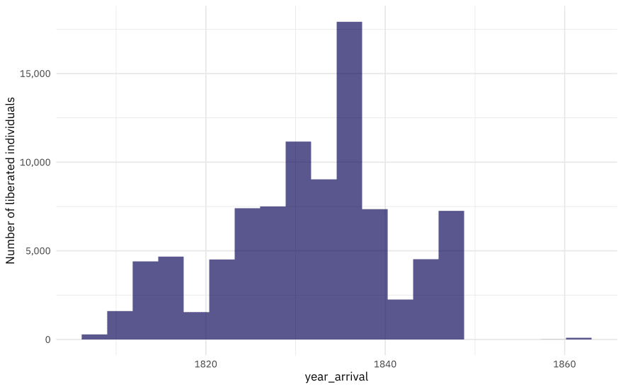
When is this data from?
african_names %>%
  ggplot(aes(year_arrival)) +
  geom_histogram(bins = 20, fill = "midnightblue", alpha = 0.7) +
  scale_y_continuous(labels = scales::comma_format()) +
  labs(y = "Number of liberated individuals")
What is the pattern of missing data?
library(naniar)

african_names %>%
  select(gender, age, height, year_arrival) %>%
  gg_miss_upset()
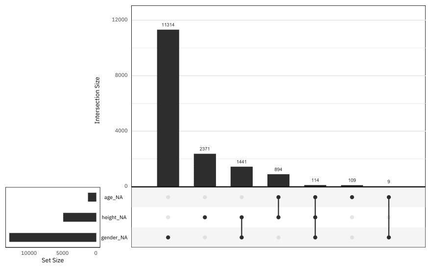
Gender has the highest proportion of missing data, and there is not much data missing from the age column. Fortunately for our attempt to impute missing values, not many rows have all three of these missing.
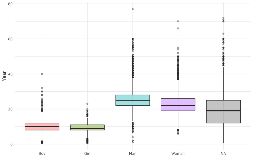
What is the relationship between gender and year of arrival?
african_names %>%
  ggplot(aes(gender, year_arrival, fill = gender)) +
  geom_boxplot(alpha = 0.4, show.legend = FALSE) +
  labs(x = NULL, y = "Year")
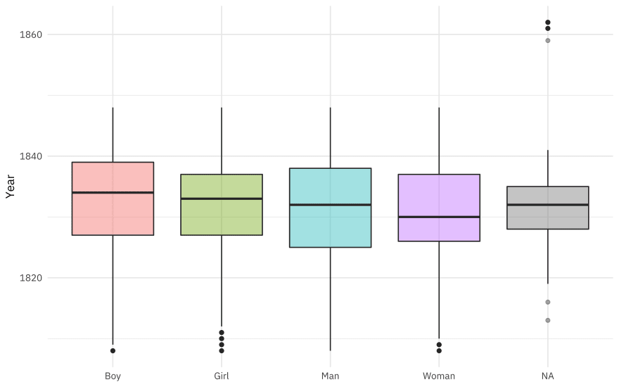
Gender was coded as both man/woman and boy/girl, but there is a fair amount of overlap in ages (children coded as “man”, for example).
african_names %>%
  ggplot(aes(gender, age, fill = gender)) +
  geom_boxplot(alpha = 0.4, show.legend = FALSE) +
  labs(x = NULL, y = "Year")
What is the relationship between age and year of arrival?
african_names %>%
  filter(year_arrival < 1850) %>%
  group_by(year_arrival) %>%
  summarise(age = mean(age, na.rm = TRUE)) %>%
  ggplot(aes(year_arrival, age)) +
  geom_line(alpha = 0.6, size = 1.5) +
  geom_smooth(method = "lm") +
  scale_y_continuous(limits = c(0, NA)) +
  labs(x = NULL, y = "Mean age")

Overall, the age is drifting up slightly, although the previous plot on boys/girls/men/women calls this into question. We can use modeling to explore this better.
One of the most unique and valuable characteristics of this dataset is the names. We can make a scatterplot to understand more about the distribution of ages and year of arrival.
library(ggrepel)

african_names %>%
  group_by(name) %>%
  summarise(
    n = n(),
    age = mean(age, na.rm = TRUE),
    year_arrival = mean(year_arrival, na.rm = TRUE)
  ) %>%
  ungroup() %>%
  arrange(-n) %>%
  filter(n > 30) %>%
  ggplot(aes(year_arrival, age)) +
  geom_text_repel(aes(label = name), size = 3, family = "IBMPlexSans") +
  geom_point(aes(size = n), color = "midnightblue", alpha = 0.7) +
  labs(
    x = "Mean year of arrival", y = "Mean age",
    size = "Number of people",
    title = "Age and year of arrival for most common names of transported captives",
    caption = "African Names Database from slavevoyages.org"
  )

I’m looking forward to how else folks explore this #TidyTuesday dataset and share on Twitter.
Impute missing data
Our modeling goal is to estimate whether some characteristics, say age and gender, of trafficked Africans changed during this time period. Some data is missing, so let’s try to impute gender and age, with the help of height. When we do imputation, we aren’t adding new information to our dataset, but we are using the patterns in our dataset so that we don’t have to throw away the data that have some variables missing.
First, let’s filter to only the data from before 1850 and recode the gender variable.
liberated_df <- african_names %>%
  filter(year_arrival < 1850) %>%
  mutate(gender = case_when(
    gender == "Boy" ~ "Man",
    gender == "Girl" ~ "Woman",
    TRUE ~ gender
  )) %>%
  mutate_if(is.character, factor)

liberated_df


## # A tibble: 91,394 x 11
## id voyage_id name gender age height ship_name year_arrival
## <dbl> <dbl> <fct> <fct> <dbl> <dbl> <fct> <dbl>
## 1 1 2314 Bora Man 30 62.5 NS de Re… 1819
## 2 2 2315 Flam Man 30 64 Fabiana 1819
## 3 3 2315 Dee Man 28 65 Fabiana 1819
## 4 4 2315 Pao Man 22 62.5 Fabiana 1819
## 5 5 2315 Mufa Man 16 59 Fabiana 1819
## 6 6 2315 Latty Man 22 67.5 Fabiana 1819
## 7 7 2315 So Man 20 62 Fabiana 1819
## 8 8 2315 Trua Man 30 65.5 Fabiana 1819
## 9 9 2315 Tou Man 18 61.5 Fabiana 1819
## 10 10 2315 Quaco Man 23 62 Fabiana 1819
## # … with 91,384 more rows, and 3 more variables: port_disembark <fct>,
## # port_embark <fct>, country_origin <fct>
Next, let’s impute the missing data using a recipe.
library(recipes)

impute_rec <- recipe(year_arrival ~ gender + age + height, data = liberated_df) %>%
  step_meanimpute(height) %>%
  step_knnimpute(all_predictors())
Let’s walk through the steps in this recipe.
- First, we must tell the
recipe()what’s going on with our model what data we are using (notice we did not split into training and testing, because of our specific modeling goals). - Next, we impute the missing values for height with the mean value for height. Height has a low value of missingness, and we are only going to use it to impute age and gender, not for modeling.
- Next, we impute the missing values for age and gender using a nearest neighbors model with all three predictors.
Once we have the recipe defined, we can estimate the parameters needed to apply it using prep(). In this case, that means finding the mean for height (fast) and training the nearest neighbor model to find gender and age (not so fast). Then we can use juice() to get that imputed data back out. (If we wanted to apply the recipe to other data, like new data we hadn’t seen before, we would use bake() instead.)
imputed <- prep(impute_rec) %>% juice()
How did the imputation turn out?
summary(liberated_df$age)


## Min. 1st Qu. Median Mean 3rd Qu. Max. NA's
## 0.50 11.00 20.00 18.89 26.00 77.00 1030


summary(imputed$age)


## Min. 1st Qu. Median Mean 3rd Qu. Max.
## 0.50 11.00 19.00 18.77 26.00 77.00


summary(liberated_df$gender)


## Man Woman NA's
## 52723 25889 12782


summary(imputed$gender)


## Man Woman
## 60992 30402
No more NA values, and the distributions look about the same. I like to keep in mind that the point of imputation like this is to be able to use the information we have in the dataset without throwing it away, which feels especially important when dealing with historical data on individuals who experienced enslavement.
Fit a model
The distribution of year of arrival was a bit wonky, so that is good to keep in mind when training a linear model.
fit_lm <- lm(year_arrival ~ gender + age, data = imputed)
We can check out the model results.
summary(fit_lm)


##
## Call:
## lm(formula = year_arrival ~ gender + age, data = imputed)
##
## Residuals:
## Min 1Q Median 3Q Max
## -23.7206 -5.3343 0.9842 5.6828 17.0903
##
## Coefficients:
## Estimate Std. Error t value Pr(>|t|)
## (Intercept) 1.832e+03 8.163e-02 22440.485 < 2e-16 ***
## genderWoman -3.014e-01 6.724e-02 -4.482 7.40e-06 ***
## age -2.123e-02 3.665e-03 -5.793 6.95e-09 ***
## ---
## Signif. codes: 0 ' ***' 0.001 '**' 0.01 '*' 0.05 '.' 0.1 ' ' 1
##
## Residual standard error: 9.476 on 91391 degrees of freedom
## Multiple R-squared: 0.0005149,   Adjusted R-squared: 0.000493
## F-statistic: 23.54 on 2 and 91391 DF, p-value: 6.012e-11


tidy(fit_lm) %>%
  kable(digits = 3)
| term | estimate | std.error | statistic | p.value |
|---|---|---|---|---|
| (Intercept) | 1831.869 | 0.082 | 22440.485 | 0 |
| genderWoman | -0.301 | 0.067 | -4.482 | 0 |
| age | -0.021 | 0.004 | -5.793 | 0 |
During the years (about 1810 to 1850) included here, as time passed, there were some gradual shifts in the population of who was found on (i.e. liberated from) these slave ships.
- There is evidence for a modest shift to younger ages as time passed. (The plot showing increasing age with time was, it turns out, an example of Simpson’s paradox.)
- In the earlier years, there were more proportionally more women while in the later years, there were proportionally more men.
I am very open to feedback on how to engage on these topics better, especially from folks who are personally impacted by this part of our history.


Top comments (1)
Finally some good old R code that i can understand. Thank you!!!