Lately I’ve been publishing screencasts demonstrating how to use the tidymodels framework, from starting out with first modeling steps to tuning more complex models. Today’s screencast walks through a detailed model analysis from beginning to end, with important feature engineering steps and several model types, using this week’s #TidyTuesday dataset on Himalayan climbing expeditions.
Here is the code I used in the video, for those who prefer reading instead of or in addition to video.
Explore the data
Our modeling goal is to predict the probability of an Himalayan expedition member surviving or dying based on characteristics of the person and climbing expedition from this week’s #TidyTuesday dataset. This dataset gives us the opportunity to talk about feature engineering steps like subsampling for class imbalance (many more people survive than die) and imputing missing data (lots of expedition members are missing age, for example).
Let’s start by reading in the data.
library(tidyverse)
members <- read_csv("https://raw.githubusercontent.com/rfordatascience/tidytuesday/master/data/2020/2020-09-22/members.csv")

members


## # A tibble: 76,519 x 21
## expedition_id member_id peak_id peak_name year season sex age
## <chr> <chr> <chr> <chr> <dbl> <chr> <chr> <dbl>
## 1 AMAD78301 AMAD7830… AMAD Ama Dabl… 1978 Autumn M 40
## 2 AMAD78301 AMAD7830… AMAD Ama Dabl… 1978 Autumn M 41
## 3 AMAD78301 AMAD7830… AMAD Ama Dabl… 1978 Autumn M 27
## 4 AMAD78301 AMAD7830… AMAD Ama Dabl… 1978 Autumn M 40
## 5 AMAD78301 AMAD7830… AMAD Ama Dabl… 1978 Autumn M 34
## 6 AMAD78301 AMAD7830… AMAD Ama Dabl… 1978 Autumn M 25
## 7 AMAD78301 AMAD7830… AMAD Ama Dabl… 1978 Autumn M 41
## 8 AMAD78301 AMAD7830… AMAD Ama Dabl… 1978 Autumn M 29
## 9 AMAD79101 AMAD7910… AMAD Ama Dabl… 1979 Spring M 35
## 10 AMAD79101 AMAD7910… AMAD Ama Dabl… 1979 Spring M 37
## # … with 76,509 more rows, and 13 more variables: citizenship <chr>,
## # expedition_role <chr>, hired <lgl>, highpoint_metres <dbl>, success <lgl>,
## # solo <lgl>, oxygen_used <lgl>, died <lgl>, death_cause <chr>,
## # death_height_metres <dbl>, injured <lgl>, injury_type <chr>,
## # injury_height_metres <dbl>
On the video, I walk through the results of skimr::skim(), and notice which variables have missing data, how many unique values there are for variables like citizenship or mountain peak, and so forth.
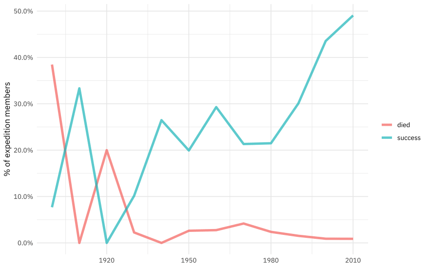
How has the rate of expedition success and member death changed over time?
members %>%
  group_by(year = 10 * (year %/% 10)) %>%
  summarise(
    died = mean(died),
    success = mean(success)
  ) %>%
  pivot_longer(died:success, names_to = "outcome", values_to = "percent") %>%
  ggplot(aes(year, percent, color = outcome)) +
  geom_line(alpha = 0.7, size = 1.5) +
  scale_y_continuous(labels = scales::percent_format()) +
  labs(x = NULL, y = "% of expedition members", color = NULL)
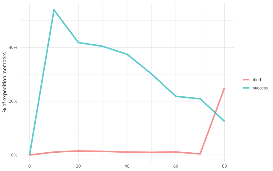
Is there a relationship between the expedition member’s age and success of the expedition or death? We can use the same code but just switch out year for age.
members %>%
  group_by(age = 10 * (age %/% 10)) %>%
  summarise(
    died = mean(died),
    success = mean(success)
  ) %>%
  pivot_longer(died:success, names_to = "outcome", values_to = "percent") %>%
  ggplot(aes(age, percent, color = outcome)) +
  geom_line(alpha = 0.7, size = 1.5) +
  scale_y_continuous(labels = scales::percent_format()) +
  labs(x = NULL, y = "% of expedition members", color = NULL)
Are people more likely to die on unsuccessful expeditions?
members %>%
  count(success, died) %>%
  group_by(success) %>%
  mutate(percent = scales::percent(n / sum(n))) %>%
  kable(
    col.names = c("Expedition success", "Died", "Number of people", "% of people"),
    align = "llrr"
  )
| Expedition success | Died | Number of people | % of people |
|---|---|---|---|
| FALSE | FALSE | 46452 | 98% |
| FALSE | TRUE | 868 | 2% |
| TRUE | FALSE | 28961 | 99% |
| TRUE | TRUE | 238 | 1% |
We can use a similar approach to see how different the rates of death are on different peaks in the Himalayas.
members %>%
  filter(!is.na(peak_name)) %>%
  mutate(peak_name = fct_lump(peak_name, prop = 0.05)) %>%
  count(peak_name, died) %>%
  group_by(peak_name) %>%
  mutate(percent = scales::percent(n / sum(n))) %>%
  kable(
    col.names = c("Peak", "Died", "Number of people", "% of people"),
    align = "llrr"
  )
| Peak | Died | Number of people | % of people |
|---|---|---|---|
| Ama Dablam | FALSE | 8374 | 100% |
| Ama Dablam | TRUE | 32 | 0% |
| Cho Oyu | FALSE | 8838 | 99% |
| Cho Oyu | TRUE | 52 | 1% |
| Everest | FALSE | 21507 | 99% |
| Everest | TRUE | 306 | 1% |
| Manaslu | FALSE | 4508 | 98% |
| Manaslu | TRUE | 85 | 2% |
| Other | FALSE | 32171 | 98% |
| Other | TRUE | 631 | 2% |
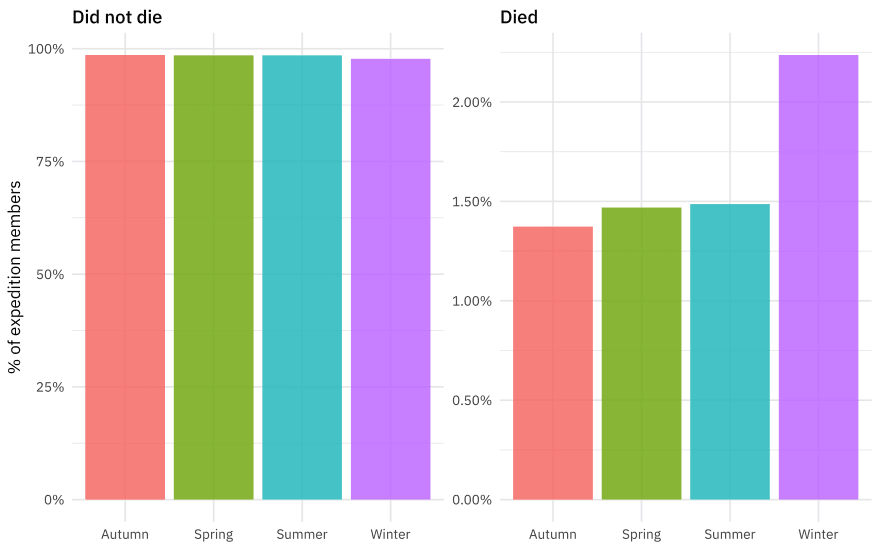
Let’s make one last exploratory plot and look at seasons. How much difference is there in survival across the four seasons?
members %>%
  filter(season != "Unknown") %>%
  count(season, died) %>%
  group_by(season) %>%
  mutate(
    percent = n / sum(n),
    died = case_when(
      died ~ "Died",
      TRUE ~ "Did not die"
    )
  ) %>%
  ggplot(aes(season, percent, fill = season)) +
  geom_col(alpha = 0.8, position = "dodge", show.legend = FALSE) +
  scale_y_continuous(labels = scales::percent_format()) +
  facet_wrap(~died, scales = "free") +
  labs(x = NULL, y = "% of expedition members")
There are lots more great examples of #TidyTuesday EDA out there to explore on Twitter! Let’s now create the dataset that we’ll use for modeling by filtering on some of the variables and transforming some variables to a be factors. There are still lots of NA values for age but we are going to impute those.
members_df <- members %>%
  filter(season != "Unknown", !is.na(sex), !is.na(citizenship)) %>%
  select(peak_id, year, season, sex, age, citizenship, hired, success, died) %>%
  mutate(died = case_when(
    died ~ "died",
    TRUE ~ "survived"
  )) %>%
  mutate_if(is.character, factor) %>%
  mutate_if(is.logical, as.integer)

members_df


## # A tibble: 76,507 x 9
## peak_id year season sex age citizenship hired success died
## <fct> <dbl> <fct> <fct> <dbl> <fct> <int> <int> <fct>
## 1 AMAD 1978 Autumn M 40 France 0 0 survived
## 2 AMAD 1978 Autumn M 41 France 0 0 survived
## 3 AMAD 1978 Autumn M 27 France 0 0 survived
## 4 AMAD 1978 Autumn M 40 France 0 0 survived
## 5 AMAD 1978 Autumn M 34 France 0 0 survived
## 6 AMAD 1978 Autumn M 25 France 0 0 survived
## 7 AMAD 1978 Autumn M 41 France 0 0 survived
## 8 AMAD 1978 Autumn M 29 France 0 0 survived
## 9 AMAD 1979 Spring M 35 USA 0 0 survived
## 10 AMAD 1979 Spring M 37 W Germany 0 1 survived
## # … with 76,497 more rows
Build a model
We can start by loading the tidymodels metapackage, and splitting our data into training and testing sets.
library(tidymodels)

set.seed(123)
members_split <- initial_split(members_df, strata = died)
members_train <- training(members_split)
members_test <- testing(members_split)
We are going to use resampling to evaluate model performance, so let’s get those resampled sets ready.
set.seed(123)
members_folds <- vfold_cv(members_train, strata = died)
members_folds


## # 10-fold cross-validation using stratification
## # A tibble: 10 x 2
## splits id
## <list> <chr>
## 1 <split [51.6K/5.7K]> Fold01
## 2 <split [51.6K/5.7K]> Fold02
## 3 <split [51.6K/5.7K]> Fold03
## 4 <split [51.6K/5.7K]> Fold04
## 5 <split [51.6K/5.7K]> Fold05
## 6 <split [51.6K/5.7K]> Fold06
## 7 <split [51.6K/5.7K]> Fold07
## 8 <split [51.6K/5.7K]> Fold08
## 9 <split [51.6K/5.7K]> Fold09
## 10 <split [51.6K/5.7K]> Fold10
Next we build a recipe for data preprocessing.
- First, we must tell the
recipe()what our model is going to be (using a formula here) and what our training data is. - Next, we impute the missing values for
ageusing the median age in the training data set. There are more complex steps available for imputation, but we’ll stick with a straightforward option here. - Next, we use
step_other()to collapse categorical levels for peak and citizenship. Before this step, there were hundreds of values in each variable. - After this, we can create indicator variables for the non-numeric, categorical values, except for the outcome
diedwhich we need to keep as a factor. - Finally, there are many more people who survived their expedition than who died (thankfully) so we will use
step_smote()to balance the classes.
The object members_rec is a recipe that has not been trained on data yet (for example, which categorical levels should be collapsed has not been calculated).
library(themis)

members_rec <- recipe(died ~ ., data = members_train) %>%
  step_medianimpute(age) %>%
  step_other(peak_id, citizenship) %>%
  step_dummy(all_nominal(), -died) %>%
  step_smote(died)

members_rec


## Data Recipe
##
## Inputs:
##
## role #variables
## outcome 1
## predictor 8
##
## Operations:
##
## Median Imputation for age
## Collapsing factor levels for peak_id, citizenship
## Dummy variables from all_nominal(), -died
## SMOTE based on died
We’re going to use this recipe in a workflow() so we don’t need to stress a lot about whether to prep() or not. If you want to explore the what the recipe is doing to your data, you can first prep() the recipe to estimate the parameters needed for each step and then bake(new_data = NULL) to pull out the training data with those steps applied.
Let’s compare two different models, a logistic regression model and a random forest model; these are the same two models I used in the post on the Palmer penguins. We start by creating the model specifications.
glm_spec <- logistic_reg() %>%
  set_engine("glm")

glm_spec


## Logistic Regression Model Specification (classification)
##
## Computational engine: glm


rf_spec <- rand_forest(trees = 1000) %>%
  set_mode("classification") %>%
  set_engine("ranger")

rf_spec


## Random Forest Model Specification (classification)
##
## Main Arguments:
## trees = 1000
##
## Computational engine: ranger
Next let’s start putting together a tidymodels workflow(), a helper object to help manage modeling pipelines with pieces that fit together like Lego blocks. Notice that there is no model yet: Model: None.
members_wf <- workflow() %>%
  add_recipe(members_rec)

members_wf


## ══ Workflow ═══════════════════════════════════════════════════════════════════════════════════════════
## Preprocessor: Recipe
## Model: None
##
## ── Preprocessor ───────────────────────────────────────────────────────────────────────────────────────
## 4 Recipe Steps
##
## ● step_medianimpute()
## ● step_other()
## ● step_dummy()
## ● step_smote()
Now we can add a model, and the fit to each of the resamples. First, we can fit the logistic regression model. Let’s set a non-default metric set so we can add sensitivity and specificity.
members_metrics <- metric_set(roc_auc, accuracy, sensitivity, specificity)

doParallel::registerDoParallel()
glm_rs <- members_wf %>%
  add_model(glm_spec) %>%
  fit_resamples(
    resamples = members_folds,
    metrics = members_metrics,
    control = control_resamples(save_pred = TRUE)
  )

glm_rs


## # Resampling results
## # 10-fold cross-validation using stratification
## # A tibble: 10 x 5
## splits id .metrics .notes .predictions
## <list> <chr> <list> <list> <list>
## 1 <split [51.6K/5.7K… Fold01 <tibble [4 × 3… <tibble [0 × … <tibble [5,739 × 5…
## 2 <split [51.6K/5.7K… Fold02 <tibble [4 × 3… <tibble [0 × … <tibble [5,738 × 5…
## 3 <split [51.6K/5.7K… Fold03 <tibble [4 × 3… <tibble [0 × … <tibble [5,738 × 5…
## 4 <split [51.6K/5.7K… Fold04 <tibble [4 × 3… <tibble [0 × … <tibble [5,738 × 5…
## 5 <split [51.6K/5.7K… Fold05 <tibble [4 × 3… <tibble [0 × … <tibble [5,738 × 5…
## 6 <split [51.6K/5.7K… Fold06 <tibble [4 × 3… <tibble [0 × … <tibble [5,738 × 5…
## 7 <split [51.6K/5.7K… Fold07 <tibble [4 × 3… <tibble [0 × … <tibble [5,738 × 5…
## 8 <split [51.6K/5.7K… Fold08 <tibble [4 × 3… <tibble [0 × … <tibble [5,738 × 5…
## 9 <split [51.6K/5.7K… Fold09 <tibble [4 × 3… <tibble [0 × … <tibble [5,738 × 5…
## 10 <split [51.6K/5.7K… Fold10 <tibble [4 × 3… <tibble [0 × … <tibble [5,738 × 5…
Second, we can fit the random forest model.
rf_rs <- members_wf %>%
  add_model(rf_spec) %>%
  fit_resamples(
    resamples = members_folds,
    metrics = members_metrics,
    control = control_resamples(save_pred = TRUE)
  )

rf_rs


## # Resampling results
## # 10-fold cross-validation using stratification
## # A tibble: 10 x 5
## splits id .metrics .notes .predictions
## <list> <chr> <list> <list> <list>
## 1 <split [51.6K/5.7K… Fold01 <tibble [4 × 3… <tibble [0 × … <tibble [5,739 × 5…
## 2 <split [51.6K/5.7K… Fold02 <tibble [4 × 3… <tibble [0 × … <tibble [5,738 × 5…
## 3 <split [51.6K/5.7K… Fold03 <tibble [4 × 3… <tibble [0 × … <tibble [5,738 × 5…
## 4 <split [51.6K/5.7K… Fold04 <tibble [4 × 3… <tibble [0 × … <tibble [5,738 × 5…
## 5 <split [51.6K/5.7K… Fold05 <tibble [4 × 3… <tibble [0 × … <tibble [5,738 × 5…
## 6 <split [51.6K/5.7K… Fold06 <tibble [4 × 3… <tibble [0 × … <tibble [5,738 × 5…
## 7 <split [51.6K/5.7K… Fold07 <tibble [4 × 3… <tibble [0 × … <tibble [5,738 × 5…
## 8 <split [51.6K/5.7K… Fold08 <tibble [4 × 3… <tibble [0 × … <tibble [5,738 × 5…
## 9 <split [51.6K/5.7K… Fold09 <tibble [4 × 3… <tibble [0 × … <tibble [5,738 × 5…
## 10 <split [51.6K/5.7K… Fold10 <tibble [4 × 3… <tibble [0 × … <tibble [5,738 × 5…
We have fit each of our candidate models to our resampled training set!
Evaluate model
Now let’s check out how we did.
collect_metrics(glm_rs)


## # A tibble: 4 x 5
## .metric .estimator mean n std_err
## <chr> <chr> <dbl> <int> <dbl>
## 1 accuracy binary 0.619 10 0.00230
## 2 roc_auc binary 0.705 10 0.00721
## 3 sens binary 0.678 10 0.0139
## 4 spec binary 0.619 10 0.00243
Well, this is middling but at least mostly consistent for the positive and negative classes. The function collect_metrics() extracts and formats the .metrics column from resampling results like the ones we have here.
collect_metrics(rf_rs)


## # A tibble: 4 x 5
## .metric .estimator mean n std_err
## <chr> <chr> <dbl> <int> <dbl>
## 1 accuracy binary 0.972 10 0.000514
## 2 roc_auc binary 0.746 10 0.00936
## 3 sens binary 0.164 10 0.0125
## 4 spec binary 0.984 10 0.000499
The accuracy is great but that sensitivity… YIKES! The random forest model has not done a great job of learning how to recognize both classes, even with our oversampling strategy. Let’s dig deeper into how these models are doing to see this more. For example, how are they predicting the two classes?
glm_rs %>%
  conf_mat_resampled()


## # A tibble: 4 x 3
## Prediction Truth Freq
## <fct> <fct> <dbl>
## 1 died died 55.5
## 2 died survived 2157.
## 3 survived died 26.5
## 4 survived survived 3499.


rf_rs %>%
  conf_mat_resampled()


## # A tibble: 4 x 3
## Prediction Truth Freq
## <fct> <fct> <dbl>
## 1 died died 13.5
## 2 died survived 89.9
## 3 survived died 68.5
## 4 survived survived 5566.
The random forest model is quite bad at identifying which expedition members died, while the logistic regression model does about the same for both classes.
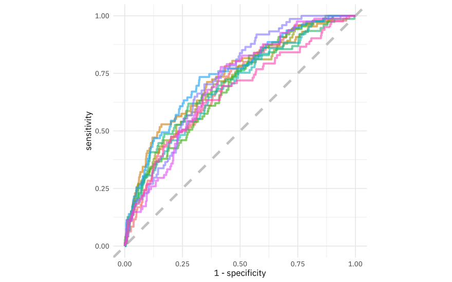
We can also make an ROC curve.
glm_rs %>%
  collect_predictions() %>%
  group_by(id) %>%
  roc_curve(died, .pred_died) %>%
  ggplot(aes(1 - specificity, sensitivity, color = id)) +
  geom_abline(lty = 2, color = "gray80", size = 1.5) +
  geom_path(show.legend = FALSE, alpha = 0.6, size = 1.2) +
  coord_equal()
It is finally time for us to return to the testing set. Notice that we have not used the testing set yet during this whole analysis; to compare and assess models we used resamples of the training set. Let’s fit one more time to the training data and evaluate on the testing data using the function last_fit().
members_final <- members_wf %>%
  add_model(glm_spec) %>%
  last_fit(members_split)

members_final


## # Resampling results
## # Manual resampling
## # A tibble: 1 x 6
## splits id .metrics .notes .predictions .workflow
## <list> <chr> <list> <list> <list> <list>
## 1 <split [57.4K… train/test… <tibble [2 … <tibble [0… <tibble [19,126… <workflo…
The metrics and predictions here are on the testing data.
collect_metrics(members_final)


## # A tibble: 2 x 3
## .metric .estimator .estimate
## <chr> <chr> <dbl>
## 1 accuracy binary 0.619
## 2 roc_auc binary 0.689


collect_predictions(members_final) %>%
  conf_mat(died, .pred_class)


## Truth
## Prediction died survived
## died 196 7204
## survived 90 11636
The coefficients (which we can get out using tidy()) have been estimated using the training data. If we use exponentiate = TRUE, we have odds ratios.
members_final %>%
  pull(.workflow) %>%
  pluck(1) %>%
  tidy(exponentiate = TRUE) %>%
  arrange(estimate) %>%
  kable(digits = 3)
| term | estimate | std.error | statistic | p.value |
|---|---|---|---|---|
| (Intercept) | 0.000 | 0.944 | -57.309 | 0.000 |
| peak_id_MANA | 0.220 | 0.042 | -35.769 | 0.000 |
| peak_id_other | 0.223 | 0.034 | -43.635 | 0.000 |
| peak_id_EVER | 0.294 | 0.036 | -33.641 | 0.000 |
| hired | 0.497 | 0.054 | -12.928 | 0.000 |
| sex_M | 0.536 | 0.029 | -21.230 | 0.000 |
| citizenship_other | 0.612 | 0.032 | -15.299 | 0.000 |
| citizenship_Japan | 0.739 | 0.038 | -7.995 | 0.000 |
| season_Winter | 0.747 | 0.041 | -7.180 | 0.000 |
| citizenship_Nepal | 0.776 | 0.062 | -4.128 | 0.000 |
| peak_id_CHOY | 0.865 | 0.043 | -3.404 | 0.001 |
| season_Spring | 0.905 | 0.016 | -6.335 | 0.000 |
| age | 0.991 | 0.001 | -12.129 | 0.000 |
| year | 1.029 | 0.000 | 59.745 | 0.000 |
| citizenship_USA | 1.334 | 0.043 | 6.759 | 0.000 |
| citizenship_UK | 1.419 | 0.045 | 7.858 | 0.000 |
| success | 2.099 | 0.016 | 46.404 | 0.000 |
| season_Summer | 7.142 | 0.092 | 21.433 | 0.000 |
We can also visualize these results.
members_final %>%
  pull(.workflow) %>%
  pluck(1) %>%
  tidy() %>%
  filter(term != "(Intercept)") %>%
  ggplot(aes(estimate, fct_reorder(term, estimate))) +
  geom_vline(xintercept = 0, color = "gray50", lty = 2, size = 1.2) +
  geom_errorbar(aes(
    xmin = estimate - std.error,
    xmax = estimate + std.error
  ),
  width = .2, color = "gray50", alpha = 0.7
  ) +
  geom_point(size = 2, color = "#85144B") +
  labs(y = NULL, x = "Coefficent from logistic regression")
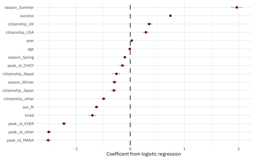
- The features with coefficients on the positive side (like climbing in summer, being on a successful expedition, or being from the UK or US) are associated with surviving.
- The features with coefficients on the negative side (like climbing specific peaks including Everest, being one of the hired members of a expedition, or being a man) are associated with dying.
Remember that we have to interpret model coefficients like this in light of the predictive accuracy of our model, which was somewhat middling; there are more factors at play in who survives these expeditions than what we have accounted for in the model directly. Also note that we see evidence in this model for how dangerous it is to be a native Sherpa climber in Nepal, hired as an expedition member, as pointed out in this week’s #TidyTuesday README.


Top comments (0)