
This is the latest in my series of screencasts demonstrating how to use the tidymodels packages, from just starting out to tuning more complex models with many hyperparameters. Today’s screencast walks through how to use bootstrap resampling, with this week’s #TidyTuesday dataset on CEO departures. 👋
Here is the code I used in the video, for those who prefer reading instead of or in addition to video.
Explore data
Our modeling goal is to estimate how involuntary CEO departures are changing with time. Let’s start by reading in the data.
library(tidyverse)

departures_raw <- read_csv("https://raw.githubusercontent.com/rfordatascience/tidytuesday/master/data/2021/2021-04-27/departures.csv")
How are involuntary departures changing with time? What about the rest of the CEO departures?
departures_raw %>%
  filter(departure_code < 9) %>%
  mutate(involuntary = if_else(departure_code %in% 3:4, "involuntary", "other")) %>%
  filter(fyear > 1995, fyear < 2019) %>%
  count(fyear, involuntary) %>%
  ggplot(aes(fyear, n, color = involuntary)) +
  geom_line(size = 1.2, alpha = 0.5) +
  geom_point(size = 2) +
  geom_smooth(method = "lm", lty = 2) +
  scale_y_continuous(limits = c(0, NA)) +
  labs(x = NULL, y = "Number of CEO departures", color = NULL)
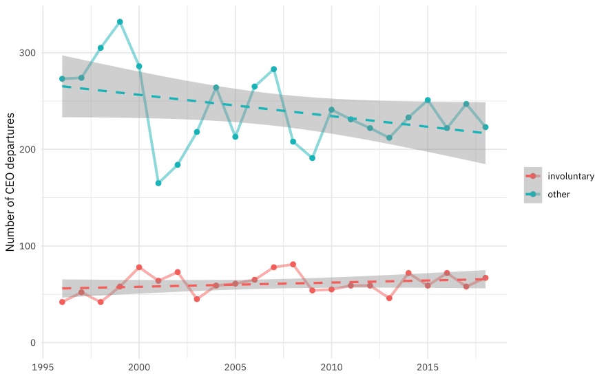
Looks like proportionally more departures are involuntary over time, but that is what we’ll work on estimating. Let’s create a data set to use for modeling.
departures <- departures_raw %>%
  filter(departure_code < 9) %>%
  mutate(involuntary = if_else(departure_code %in% 3:4, "involuntary", "other")) %>%
  filter(fyear > 1995, fyear < 2019)

departures


## # A tibble: 6,942 x 20
## dismissal_datase… coname gvkey fyear co_per_rol exec_fullname departure_code
## <dbl> <chr> <dbl> <dbl> <dbl> <chr> <dbl>
## 1 559043 SONICB… 27903 2002 -1 L. Gregory B… 7
## 2 12 AMERIC… 1045 1997 1 Robert L. Cr… 5
## 3 13 AMERIC… 1045 2002 3 Donald J. Ca… 3
## 4 31 ABBOTT… 1078 1998 6 Duane L. Bur… 5
## 5 43 ADVANC… 1161 2001 11 Walter Jerem… 5
## 6 51 AETNA … 1177 1997 16 Ronald Edwar… 5
## 7 63 AHMANS… 1194 1997 22 Charles R. R… 7
## 8 65 AIR PR… 1209 2000 28 Harold A. Wa… 5
## 9 76 ALBERT… 1239 2007 34 Howard B. Be… 5
## 10 78 ALBERT… 1240 2000 38 Gary Glenn M… 3
## # … with 6,932 more rows, and 13 more variables: ceo_dismissal <dbl>,
## # interim_coceo <chr>, tenure_no_ceodb <dbl>, max_tenure_ceodb <dbl>,
## # fyear_gone <dbl>, leftofc <dttm>, still_there <chr>, notes <chr>,
## # sources <chr>, eight_ks <chr>, cik <dbl>, _merge <chr>, involuntary <chr>
Bootstrapping a model
We can count up the two kinds of departures per financial year and fit the model once, for the whole data set.
library(broom)

df <- departures %>%
  count(fyear, involuntary) %>%
  pivot_wider(names_from = involuntary, values_from = n)

mod <- glm(cbind(involuntary, other) ~ fyear, data = df, family = "binomial")
summary(mod)


##
## Call:
## glm(formula = cbind(involuntary, other) ~ fyear, family = "binomial",
## data = df)
##
## Deviance Residuals:
## Min 1Q Median 3Q Max
## -2.9858 -1.2075 -0.1947 0.7302 3.6816
##
## Coefficients:
## Estimate Std. Error z value Pr(>|z|)
## (Intercept) -33.236731 8.949722 -3.714 0.000204 ***
## fyear 0.015875 0.004459 3.560 0.000370 ***
## ---
## Signif. codes: 0 ' ***' 0.001 '**' 0.01 '*' 0.05 '.' 0.1 ' ' 1
##
## (Dispersion parameter for binomial family taken to be 1)
##
## Null deviance: 78.421 on 22 degrees of freedom
## Residual deviance: 65.722 on 21 degrees of freedom
## AIC: 200.86
##
## Number of Fisher Scoring iterations: 4


tidy(mod, exponentiate = TRUE)


## # A tibble: 2 x 5
## term estimate std.error statistic p.value
## <chr> <dbl> <dbl> <dbl> <dbl>
## 1 (Intercept) 3.68e-15 8.95 -3.71 0.000204
## 2 fyear 1.02e+ 0 0.00446 3.56 0.000370
When we use exponentiate = TRUE, we get the model coefficients on the linear scale instead of the logistic scale.
What we want to do is fit a model like this a whole bunch of times, instead of just once. Let’s create bootstrap resamples.
library(rsample)

set.seed(123)
ceo_folds <- bootstraps(departures, times = 1e3)
ceo_folds


## # Bootstrap sampling
## # A tibble: 1,000 x 2
## splits id
## <list> <chr>
## 1 <split [6942/2543]> Bootstrap0001
## 2 <split [6942/2557]> Bootstrap0002
## 3 <split [6942/2509]> Bootstrap0003
## 4 <split [6942/2554]> Bootstrap0004
## 5 <split [6942/2542]> Bootstrap0005
## 6 <split [6942/2530]> Bootstrap0006
## 7 <split [6942/2509]> Bootstrap0007
## 8 <split [6942/2553]> Bootstrap0008
## 9 <split [6942/2586]> Bootstrap0009
## 10 <split [6942/2625]> Bootstrap0010
## # … with 990 more rows
Now we need to make a function to count up the departures by year and type, fit our model, and return the coefficients we want.
fit_binom <- function(split) {
  df <- analysis(split) %>%
    count(fyear, involuntary) %>%
    pivot_wider(names_from = involuntary, values_from = n)

  mod <- glm(cbind(involuntary, other) ~ fyear, data = df, family = "binomial")
  tidy(mod, exponentiate = TRUE)
}
We can apply that function to all our bootstrap resamples with purrr::map().
boot_models <- ceo_folds %>% mutate(coef_info = map(splits, fit_binom))
boot_models


## # Bootstrap sampling
## # A tibble: 1,000 x 3
## splits id coef_info
## <list> <chr> <list>
## 1 <split [6942/2543]> Bootstrap0001 <tibble [2 × 5]>
## 2 <split [6942/2557]> Bootstrap0002 <tibble [2 × 5]>
## 3 <split [6942/2509]> Bootstrap0003 <tibble [2 × 5]>
## 4 <split [6942/2554]> Bootstrap0004 <tibble [2 × 5]>
## 5 <split [6942/2542]> Bootstrap0005 <tibble [2 × 5]>
## 6 <split [6942/2530]> Bootstrap0006 <tibble [2 × 5]>
## 7 <split [6942/2509]> Bootstrap0007 <tibble [2 × 5]>
## 8 <split [6942/2553]> Bootstrap0008 <tibble [2 × 5]>
## 9 <split [6942/2586]> Bootstrap0009 <tibble [2 × 5]>
## 10 <split [6942/2625]> Bootstrap0010 <tibble [2 × 5]>
## # … with 990 more rows
Explore results
What did we find? We can compute bootstrap confidence intervals with int_pctl().
percentile_intervals <- int_pctl(boot_models, coef_info)
percentile_intervals


## # A tibble: 2 x 6
## term .lower .estimate .upper .alpha .method
## <chr> <dbl> <dbl> <dbl> <dbl> <chr>
## 1 (Intercept) 6.03e-23 0.0000273 0.000000246 0.05 percentile
## 2 fyear 1.01e+ 0 1.02 1.03 0.05 percentile
We can also visualize the results as well.
boot_models %>%
  unnest(coef_info) %>%
  filter(term == "fyear") %>%
  ggplot(aes(estimate)) +
  geom_vline(xintercept = 1, lty = 2, color = "gray50", size = 2) +
  geom_histogram() +
  labs(
    x = "Annual increase in involuntary CEO departures",
    title = "Over this time period, CEO departures are increasingly involuntary",
    subtitle = "Each passing year corresponds to a departure being 1-2% more likely to be involuntary"
  )


Top comments (0)