
This is the latest in my series of screencasts demonstrating how to use the tidymodels packages, from starting out with first modeling steps to tuning more complex models. One change I have recently made on my blog is to remove Disqus comments. I want to say a huge THANK YOU 🙏 to everyone who ever commented on my blog before and express how much I appreciate folks’ interest and willingness to share their thoughts. Disqus was becoming frustrating for a couple of reasons, so I downloaded my archive (so I can look up any old comments in the future if needed) and then switched to utteranc.es, with help from this post by Maëlle Salmon. I believe this will work better going forward!
Today’s screencast explores how to use tidymodels for unsupervised machine learning, using this week’s #TidyTuesday data set on United Nationsl voting. 🗳
Here is the code I used in the video, for those who prefer reading instead of or in addition to video.
Explore data
This analysis is very similar to what I did last May for the #TidyTuesday data set on cocktail recipes, so take a look at both to see what is the same and what is different for the two different data sets. Our modeling goal is to use unsupervised algorithms for dimensionality reduction with United Nations voting data to understand which countries are similar.
library(tidyverse)

unvotes <- read_csv("https://raw.githubusercontent.com/rfordatascience/tidytuesday/master/data/2021/2021-03-23/unvotes.csv")
issues <- read_csv("https://raw.githubusercontent.com/rfordatascience/tidytuesday/master/data/2021/2021-03-23/issues.csv")
Let’s create a wide version of this data set via pivot_wider() to use for modeling.
unvotes_df <- unvotes %>%
  select(country, rcid, vote) %>%
  mutate(
    vote = factor(vote, levels = c("no", "abstain", "yes")),
    vote = as.numeric(vote),
    rcid = paste0("rcid_", rcid)
  ) %>%
  pivot_wider(names_from = "rcid", values_from = "vote", values_fill = 2)
Principal component analysis
This analysis only uses the recipes package, the tidymodels package for data preprocessing and feature engineering that contains functions for unsupervised methods. There are lots of options available, like step_ica() and step_kpca(), but let’s implement a basic principal component analysis.
library(recipes)

pca_rec <- recipe(~., data = unvotes_df) %>%
  update_role(country, new_role = "id") %>%
  step_normalize(all_predictors()) %>%
  step_pca(all_predictors(), num_comp = 5)

pca_prep <- prep(pca_rec)

pca_prep


## Data Recipe
##
## Inputs:
##
## role #variables
## id 1
## predictor 6202
##
## Training data contained 200 data points and no missing data.
##
## Operations:
##
## Centering and scaling for rcid_3, rcid_4, rcid_5, rcid_6, rcid_7, ... [trained]
## PCA extraction with rcid_3, rcid_4, rcid_5, rcid_6, rcid_7, ... [trained]
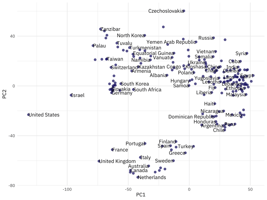
We can look at where the countries are in the principal component space by baking the prepped recipe.
bake(pca_prep, new_data = NULL) %>%
  ggplot(aes(PC1, PC2, label = country)) +
  geom_point(color = "midnightblue", alpha = 0.7, size = 2) +
  geom_text(check_overlap = TRUE, hjust = "inward", family = "IBMPlexSans") +
  labs(color = NULL)
We can look at which votes contribute to the component by tidying the prepped recipe. Let’s join the roll call votes up with the topics to see which topics contribute to the top principal components.
pca_comps <- tidy(pca_prep, 2) %>%
  filter(component %in% paste0("PC", 1:4)) %>%
  left_join(issues %>% mutate(terms = paste0("rcid_", rcid))) %>%
  filter(!is.na(issue)) %>%
  group_by(component) %>%
  top_n(8, abs(value)) %>%
  ungroup()

pca_comps %>%
  mutate(value = abs(value)) %>%
  ggplot(aes(value, fct_reorder(terms, value), fill = issue)) +
  geom_col(position = "dodge") +
  facet_wrap(~component, scales = "free_y") +
  labs(
    x = "Absolute value of contribution",
    y = NULL, fill = NULL,
    title = "What issues are most important in UN voting country differences?",
    subtitle = "Human rights and economic development votes account for the most variation"
  )
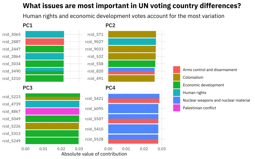
The PCA implementation did not know about the topics of the votes, but notice how the first principal component is mostly about human rights and economic development, the second principal component is mostly about colonialsim, and so on.
UMAP
To switch out for a different dimensionality reduction approach, we just need to change to a different recipe step_(). Let’s try out UMAP, a different algorithm for dimensionality reduction based on ideas from topological data analysis, which is available in the embed package.
library(embed)

umap_rec <- recipe(~., data = unvotes_df) %>%
  update_role(country, new_role = "id") %>%
  step_normalize(all_predictors()) %>%
  step_umap(all_predictors())

umap_prep <- prep(umap_rec)

umap_prep


## Data Recipe
##
## Inputs:
##
## role #variables
## id 1
## predictor 6202
##
## Training data contained 200 data points and no missing data.
##
## Operations:
##
## Centering and scaling for rcid_3, rcid_4, rcid_5, rcid_6, rcid_7, ... [trained]
## UMAP embedding for rcid_3, rcid_4, rcid_5, rcid_6, rcid_7, ... [trained]
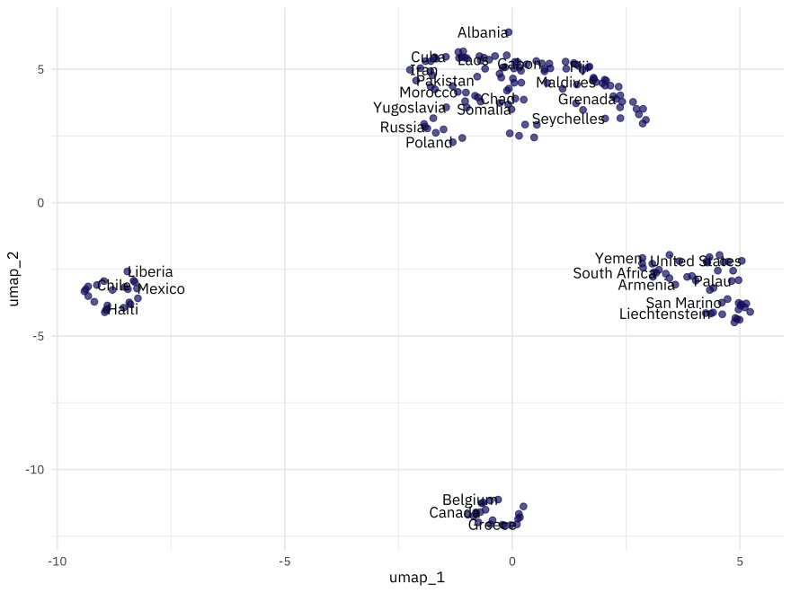
When we visualize where countries are in the space created by this dimensionality reduction approach, it looks very different!
bake(umap_prep, new_data = NULL) %>%
  ggplot(aes(umap_1, umap_2, label = country)) +
  geom_point(color = "midnightblue", alpha = 0.7, size = 2) +
  geom_text(check_overlap = TRUE, hjust = "inward", family = "IBMPlexSans") +
  labs(color = NULL)


Top comments (0)