This article was originally posted on neptune.ml/blog where you can find more in-depth articles for machine learning practitioners.
Thinking which library should you choose for hyperparameter optimization?
Been using Hyperopt for a while and feel like changing?
Just heard about Optuna and you want to see how it works?
Good!
In this article I will:
show you an example of using Optuna and Hyperopt on a real problem,
compare Optuna vs Hyperopt on API, documentation, functionality, and more,
give you my overall score and recommendation on which hyperparameter optimization library you should use.
Let’s do it.
Evaluation criteria
Ease of use and API
Options methods and hyper(hyperparameters)
- Search Space
- Optimization Methods
- Callbacks
- Persisting and Restarting
- Run Pruning
- Handling Exceptions
Documentation
Visualizations
Speed and Parallelization
Experimental Results
Ease of use and API
In this section I want to see how to run a basic hyperparameter tuning script for both libraries, see how natural and easy-to-use it is and what is the API.
Optuna
You define your search space and objective in one function.
Moreover, you sample the hyperparameters from the trial object. Because of that, the parameter space is defined at execution. For those of you who like Pytorch because of this imperative approach, Optuna will feel natural.
def objective(trial):
    params = {'learning_rate': trial.suggest_loguniform('learning_rate', 0.01, 0.5),
              'max_depth': trial.suggest_int('max_depth', 1, 30),
              'num_leaves': trial.suggest_int('num_leaves', 2, 100),
              'min_data_in_leaf': trial.suggest_int('min_data_in_leaf', 10, 1000),
              'feature_fraction': trial.suggest_uniform('feature_fraction', 0.1, 1.0),
              'subsample': trial.suggest_uniform('subsample', 0.1, 1.0)}
    return train_evaluate(params)
Then, you create the study object and optimize it. What is great is that you can choose whether you want to maximize or minimize your objective. That is useful when optimizing a metric like AUC because you don’t have to change the sign of the objective before training and then convert best results after training to get a positive score.
study = optuna.create_study(direction='Optuna > Hyperopt
maximize')
study.optimize(objective, n_trials=100)
That is it.
Everything you may want to know about the optimization is available in the study object.
What I love about Optuna is that I get to define how I want to sample my search space on-the-fly which gives me a lot of flexibility. Ability to choose a direction of optimization is also pretty nice.
If you want to see the full code example you can scroll down to the Example script.
10 / 10
Hyperopt
You start by defining your parameter search space:
SPACE = {'learning_rate':
hp.loguniform('learning_rate',np.log(0.01),np.log(0.5)),
         'max_depth':
hp.choice('max_depth', range(1, 30, 1)),
         'num_leaves':
hp.choice('num_leaves', range(2, 100, 1)),
         'subsample':
hp.uniform('subsample', 0.1, 1.0)}
Then, you create an objective function that you want to minimize. That means you will have to flip the sign of your objective for the-higher-the-better metric like AUC.
def objective(params):
    return -1.0 * train_evaluate(params)
Finally, you instantiate the Trials() object and minimize your objective on the parameter search SPACE.
trials = Trials()
_ = fmin(objective, SPACE, trials=trials, algo=tpe.suggest, max_evals=100)
…and done!
All the information about the hyperparameters that were tested and the corresponding score are kept in the trials object.
The thing that I don’t like is the fact that I need to instantiate the Trials() even in the simplest of cases. I would rather have fmin return the trials and do the instantiation by default.
9 / 10
Both libraries do a good job here but I feel that Optuna is slightly better because of the flexibility, imperative approach to sampling parameters and a bit less boilerplate.
Ease of use and API
Optuna > Hyperopt
Jump back to the evaluation criteria ->
Options, methods, and hyper(hyperparameters)
In real-life scenarios running hyperparameter optimization requires a lot of additional options away from the golden path. Areas that I am particularly interested in are:
- search space
- optimization methods/algorithms
- callbacks
- persisting and restarting parameter sweeps
- pruning unpromising runs
- handling exceptions
In this section, I will compare Optuna and Hyperopt on exactly those.
Search Space
In this section I want to compare the search space definition, flexibility in defining a complex space and sampling options for each parameter type (Float, Integer, Categorical).
Optuna
You can find sampling options for all hyperparameter types:
- for categorical parameters you can use trials.suggest_categorical
- for integers there is trials.suggest_int
- for float parameters you have trials.suggest_uniform, trials.suggest_loguniform and even, more exotic, trials.suggest_discrete_uniform
Especially for the integer parameters, you could wish for more options but it deals with most use-cases.
A great feature of this library is that you sample from the parameter space on-the-fly and you can do it however you like.
You can use if statements, you can change intervals from which you search, you can use the information from the trial object to guide your search.
def objective(trial):
    classifier_name = trial.suggest_categorical('classifier', ['SVC', 'RandomForest'])
    if classifier_name == 'SVC':
        svc_c = trial.suggest_loguniform('svc_c', 1e-10, 1e10)
        classifier_obj = sklearn.svm.SVC(C=svc_c)
    else:
        rf_max_depth = int(trial.suggest_loguniform('rf_max_depth', 2, 32))
        classifier_obj = sklearn.ensemble.RandomForestClassifier(max_depth=rf_max_depth)

    ...
This is awesome, you can do literally anything!
10 / 10
Hyperopt
Search space is where Hyperopt really gives you a ton of sampling options:
- for categorical parameters you have hp.choice
- for integers you get hp.randit, hp.quniform, hp.qloguniform and hp.qlognormal
- for floats we have hp.normal, hp.uniform, hp.lognormal and hp.loguniform
As far as I know this is the most extensive sampling functionality out there.
You define your search space before you run optimization but you can create very complex parameter spaces:
SPACE = hp.choice('classifier_type', [
    {
        'type': 'naive_bayes',
    },
    {
        'type': 'svm',
        'C': hp.lognormal('svm_C', 0, 1),
        'kernel': hp.choice('svm_kernel', [
            {'ktype': 'linear'},
            {'ktype': 'RBF', 'width': hp.lognormal('svm_rbf_width', 0, 1)},
            ]),
    },
    {
        'type': 'dtree',
        'criterion': hp.choice('dtree_criterion', ['gini', 'entropy']),
        'max_depth': hp.choice('dtree_max_depth',
            [None, hp.qlognormal('dtree_max_depth_int', 3, 1, 1)]),
        'min_samples_split': hp.qlognormal('dtree_min_samples_split', 2, 1, 1),
    },
    ])
By combining hp.choice with other sampling methods we can have conditional spaces. This is useful when you are optimizing hyperparameters for a machine learning pipeline that involves preprocessing, feature engineering and model training.
10 / 10
I have to say I like them both. I can define nested search spaces easily and I have a lot of sampling options for all the parameter types. Optuna has an imperative parameter definition, which gives more flexibility while Hyperopt has more parameter sampling options.
Search Space
Optuna = Hyperopt
Jump back to the evaluation criteria ->
Optimization methods
Both Optuna and Hyperopt are using the same optimization methods under the hood. They have:
rand.suggest (Hyperopt) and samplers.random.RandomSampler (Optuna)
Your standard random search over the parameters.
tpe.suggest (Hyperopt) and samplers.tpe.sampler.TPESampler (Optuna)
Tree of Parzen Estimators (TPE). The idea behind this method is similar to what was explained in the previous blog post about Scikit Optimize. We use a cheap surrogate model to estimate the performance of the expensive objective function on a set of parameters.
The difference between the methods used in Scikit Optimize and Tree of Parzen Estimators (TPE) is that instead of estimating the actual performance (point estimation) we want to estimate the density in the tails. We want to be able to tell whether a run will be good (right tail) or bad (left tail).
I like the following explanation taken from the AutoML_Book by amazing folks over at AutoML.org Freiburg.
Instead of modeling the probability p(y|λ) of observations y given the > configurations λ, the Tree Parzen Estimator models density functions p(λ|y < α) and p(λ|y ≥ α). Given a percentile α (usually set to 15%), the observations are divided in good observations and bad observations and simple 1-d Parzen windows are used to model the two distributions.
By using p(λ|y < α) and p(λ|y ≥ α) you can estimate the expected improvement of a parameter configuration over previous best.
Interestingly, both for Optuna and Hyperopt, there are no options to specify the α parameter in the optimizer.
Optuna
integration.SkoptSampler
Optuna lets you use samplers from Scikit-Optimize (skopt).
Skopt offers a bunch of Tree-Based methods as a choice for your surrogate model.
In order to use them you need to:
create a SkoptSampler instance specifying the parameters of the surrogate model and acquisition function in the skopt_kwargs argument,
pass the sampler instance to the optuna.create_study method
from optuna.integration import SkoptSampler

sampler = SkoptSampler(skopt_kwargs={'base_estimator':'RF',
                                     'n_random_starts':10,
                                     'base_estimator':'ET',
                                     'acq_func':'EI',
                                     'acq_func_kwargs': {'xi':0.02})
study = optuna.create_study(sampler=sampler)
study.optimize(objective, n_trials=100)
pruners.SuccessiveHalvingPruner
You can also use one of the multiarmed bandit methods called Asynchronous Successive Halving Algorithm (ASHA). If you are interested in the details please read the paper but the general idea is to:
- run a bunch of parameter configurations for some time
- prune the (half of) the least promising runs every
- run a bunch of parameter configurations for some more time
- prune the (half of) the least promising runs every
- stop when only one configuration is left
By doing so, the search can focus on the more promising runs. However, the static allocation of the budgets to configurations is a problem in practice (which a newer approach called HyperBand solves).
It is very easy to use ASHA in Optuna. Just pass a SuccesiveHalvingPruner to .create_study() and you are good to go:
from optuna.pruners import SuccessiveHalvingPruner

optuna.create_study(pruner=SuccessiveHalvingPruner())
study.optimize(objective, n_trials=100)
Nice and simple.
If you would like to learn more, you may want to check out my article about Scikit Optimize.
Overall, there are a lot of options when it comes to optimization functions right now. However, there are some important ones, like Hyperband or BOHB missing.
8 / 10
Hyperopt
atpe.suggest
Recently added, adaptive TPE was invented at ElectricBrain and it is actually a series of (not so) little improvements that they experimented with on top of TPE.
The authors explain their approach and modifications they made to TPE thoroughly in this fascinating blog post.
It is super easy to use. Instead of tpe.suggest you need to pass atpe.suggest to your fmin function.
from hyperopt import fmin, atpe

best = fmin(objective, SPACE,
            max_evals=100,
            algo=atpe.suggest)
I really like this effort to include new optimization algorithms in the library, especially since it’s a new original approach not just an integration with the existing algorithm.
Hopefully, in the future, multi-armed bandit methods like Hyperband, BOHB, or tree-based methods like SMAC3 will be included as well.
8 / 10
Optimization methods
Optuna = Hyperopt
Jump back to the evaluation criteria ->
Callbacks
In this section, I want to see how easy it is to define callbacks to monitor/snapshot/modify training after each iteration. It is useful, especially when your training is long and/or distributed.
Optuna
User callbacks are nicely supported with the callbacks argument in of the .optimize() method. Just pass a list of callables that take study and trial as input and you are good to go.
def neptune_monitor(study, trial):
    neptune.log_metric('run_score', trial.value)
    neptune.log_text('run_parameters', str(trial.params))
...
study.optimize(objective, n_trials=100, callbacks=[neptune_monitor])
Because you can access both study and trial you have all the flexibility you can possibly want to checkpoint, do early stopping or modify future search.
10 / 10
Hyperopt
There are no callbacks per se, but you can put your callback function inside the objective and it will be executed every time the objective is called.
def monitor_callback(params, score):
    neptune.send_metric('run_score', score)
    neptune.send_text('run_parameters', str(params))

def objective(params):
    score = -1.0 * train_evaluate(params)
    monitor_callback(params, score)
    return score
I don’t love it but I guess I can live with that.
6 / 10
Optuna makes it really easy with the callbacks argument while in Hyperopt you have to modify the objective.
Callbacks
Optuna > Hyperopt
Note:
If you want to monitor your Optuna experiments and log all the charts, visualizations, and results you can use Neptune helpers:
- opt.utils.neptune_monitor: logs run scores and run parameters and plots the scores so far
- opt_utils.log_study: logs best results, best param, and the study object itself
Just add this to your script:
import neptune
import neptunecontrib.monitoring.optuna as opt_utils

neptune.init('jakub-czakon/blog-hpo')
neptune.create_experiment(name='optuna sweep')

monitor = opt_utils.NeptuneMonitor()
study = optuna.create_study(direction='maximize')
study.optimize(objective, n_trials=100, callbacks=[monitor])
opt_utils.log_study(study)
Persisting and restarting
Saving and loading your hyperparameter searches can save you time, money, and can help get better results. Let’s compare both frameworks on that.
Optuna
Simply use joblib.dump to pickle the trials object.
study.optimize(objective, n_trials=100)
joblib.dump(study, 'artifacts/study.pkl')
… and you can load it later with joblib.load to restart your search.
study = joblib.load('../artifacts/study.pkl')
study.optimize(objective, n_trials=200)
That’s it.
For distributed setups, you can use the name of the study the URL to the database where your distributed study is to instantiate new study. For example:
study = optuna.create_study(
                    study_name='example-study',
                    storage='sqlite:///example.db',
                    load_if_exists=True)
Nice and easy.
More about running distributed hyperparameter optimization with Optuna in the Speed and Parallelization section.
10 / 10
Hyperopt
Similarly to Optuna use joblib.dump to pickle the trials object.
trials = Trials()
_ = fmin(objective, SPACE, trials=trials,
         algo=tpe.suggest, max_evals=100)
joblib.dump(trials, 'artifacts/hyperopt_trials.pkl')
… load it with joblib.load and restart.
trials = joblib.load('artifacts/hyperopt_trials.pkl')
_ = fmin(objective, SPACE, trials=trials,
         algo=tpe.suggest, max_evals=200)
Simple and works with no problems.
If you are optimizing hyperparameters in a distributed fashion you can load MongoTrials() object that connects to MongoDB. More about running distributed hyperparameter optimization with Hyperopt in the Speed and Parallelization section.
10 / 10
Both make it easy and get the job done.
Persisting and restarting
Optuna = Hyperopt
Jump back to the evaluation criteria ->
Run Pruning
Not all hyperparameter configurations are created equal. For some of them, you can tell very quickly that they will not produce high scores. Ideally, you would like to stop those runs as soon as possible try different parameters instead.
Optuna gives you an option to do that with Pruning Callbacks. Many machine learning frameworks are supported:
- KerasPruningCallback, TFKerasPruningCallback
- TensorFlowPruningHook
- PyTorchIgnitePruningHandler, PyTorchLightningPruningCallback
- FastAIPruningCallback
- LightGBMPruningCallback
- XGBoostPruningCallback
- and more
You can read about them in the docs.
For example, in the case of lightGBM training you would pass this callback to the lgb.train function.
def train_evaluate(X, y, params, pruning_callback=None):
    X_train, X_valid, y_train, y_valid = train_test_split(X, y, test_size=0.2, random_state=1234)

    train_data = lgb.Dataset(X_train, label=y_train)
    valid_data = lgb.Dataset(X_valid, label=y_valid, reference=train_data)

    callbacks = [pruning_callback] if pruning_callback is not None else None

    model = lgb.train(params, train_data,
                      num_boost_round=NUM_BOOST_ROUND,
                      early_stopping_rounds=EARLY_STOPPING_ROUNDS,
                      valid_sets=[valid_data],
                      valid_names=['valid'],
                      callbacks=callbacks)
    score = model.best_score['valid']['auc']
    return score

def objective(trial):
    params = {'learning_rate': trial.suggest_loguniform('learning_rate', 0.01, 0.5),
              'max_depth': trial.suggest_int('max_depth', 1, 30),
              'num_leaves': trial.suggest_int('num_leaves', 2, 100),
              'min_data_in_leaf': trial.suggest_int('min_data_in_leaf', 10, 1000),
              'feature_fraction': trial.suggest_uniform('feature_fraction', 0.1, 1.0),
              'subsample': trial.suggest_uniform('subsample', 0.1, 1.0)}

    pruning_callback = LightGBMPruningCallback(trial, 'auc', 'valid')
    return train_evaluate(params, pruning_callback)
Only Optuna gives you this option so it is a clear win.
Run Pruning
Optuna > Hyperopt
Jump back to the evaluation criteria ->
Handling Exceptions
If one of your runs fails due to the wrong parameter combination, random training error or some other problem you could lose all the parameter_configuration:score pairs evaluated so far in a study.
You can use callbacks to save this information after every iteration or use a DB to store it as explained in the Speed and Parallelization
section.
However, you may want to let this study continue even when the exception happens. To make it possible, Optuna lets you pass the allowed exceptions to the .optimize() method.
def objective(trial):
    params = {'learning_rate': trial.suggest_loguniform('learning_rate', 0.01, 0.5),
              'max_depth': trial.suggest_int('max_depth', 1, 30),
              'num_leaves': trial.suggest_int('num_leaves', 2, 100)}

    print(non_existent_variable)

    return train_evaluate(params)

study = optuna.create_study(direction='maximize')
study.optimize(objective, n_trials=100, catch=(NameError,))
Again, only Optuna supports this.
Handling Exceptions
Optuna > Hyperopt
Jump back to the evaluation criteria ->
Documentation
When you are a user of a library or a framework it is absolutely crucial to find the information you need when you need it. This is where documentation/support channels come into the picture and they can make or break a library.
Let’s see how Optuna and Hyperopt compare on that.
Optuna
It is really good.
There is a proper webpage that explains all the basic concepts and shows you where to find more information.
Also, there is complete and very easy-to-understand documentation on read-the-docs.
It contains:
- Tutorials with both simple and advanced examples
- API Reference with all the functions containing beautiful docstrings. To give you an idea imagine having charts inside of your docstrings so that you can understand what is happening inside your function better. Check out the BaseSampler if you don’t believe me.
It is also important to mention that the supporting team from Preferred Networks really takes care of this project. They respond to Github issues and the community is growing around it with great feature ideas and PRs coming in. Checkout the Github project issues section to see what is going on there.
10 / 10
Hyperopt
It was recently updated and now it is quite alright.
You can find it here.
You can easily find information about:
- how to get started
- how to define both simple and advances search spaces
- how to run the installation
- how to run Hyperopt in parallel via MongoDB or Spark
Unfortunately, there were some things that I didn’t like:
- missing API reference with the docstrings all functions/methods
- docstrings themselves are missing for most of methods/functions which forces you to read the implementation (there are some positive side effects here:) )
- no examples of using Adaptive TPE. I wasn’t sure if I am using it correctly, whether I should specify some additional (hyper)hyper parameters. Missing docstrings didn’t help me here either.
- some links to 404 in the docs.
Overall, it has improved a lot lately, but I was still a bit lost at times. I hope that with time it will get even better so stay tuned.
The good thing is, there are a lot of blog posts about it. Some of them that I found useful are:
- “Parameter Tuning with Hyperopt” by District Data Labs
- “Hyperopt tutorial for Optimizing Neural Networks Hyperparameters” by Vooban
- “On Using Hyperopt: Advanced Machine Learning” by Tanay Agrawal
- “An Introductory Example of Bayesian Optimization in Python with Hyperopt” by Will Koehrsen
The documentation is not the strongest side of this project but because it’s a classic there are a lot of resources out there.
6 / 10
Documentation
Optuna > Hyperopt
Jump back to the evaluation criteria ->
Visualizations
Visualizing hyperparameter searches can be very useful. You can gain information on interactions between parameters and see where you should search next.
That is why I want to compare visualization suits that Optuna and Hyperopt offer.
Optuna
A few great visualizations are available in the optuna.visualization module:
- plot_contour: plots parameter interactions on an interactive chart. You can choose which hyperparameters you would like to explore.
plot_contour(study, params=['learning_rate',
                            'max_depth',
                            'num_leaves',
                            'min_data_in_leaf',
                            'feature_fraction',
                            'subsample'])
- plot_optimization_history: shows the scores from all trials as well as the best score so far at each point.
plot_optimization_history(study)
- plot_parallel_coordinate: interactively visualizes the hyperparameters and scores
plot_parallel_coordinate(study)
- plot_slice: shows the evolution of the search. You can see where in the hyperparameter space your search went and which parts of the space were explored more.
plot_slice(study)
Overall, visualizations in Optuna are incredibile!
They let you zoom in on the hyperparameter interactions and help you decide on how to run your next parameter sweep. Amazing job.
10 / 10
Hyperopt
There are three visualization functions in the hyperopt.plotting module:
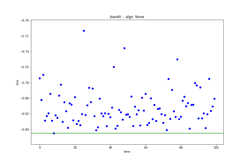
- main_plot_history: shows you the results of each iteration and highlights the best score.
main_plot_history(trials)
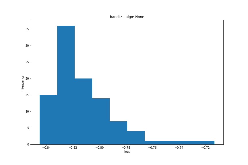
- main_plot_histogram: shows you the histogram of results over all iterations.
main_plot_histogram(trials)
- main_plot_vars: I don’t really know what it does as I couldn’t get it to run and there were no docstrings nor examples (again, the documentation is far from perfect).
Summing up, there are some basic visualization utilities but they are not super useful.
3 / 10
I am very impressed by the visualizations available in Optuna. Useful, interactive, and beautiful.
Visualizations
Optuna > Hyperopt
Note:
If you want to play with those visualizations you can use the study object that I saved as ‘study.pkl’ for each experiment.
For example go to artifacts of this one.
Jump back to the evaluation criteria ->
Speed and Parallelization
When it comes to hyperparameter optimization, being able to distribute your training on your machine or many machines (cluster) can be crucial.
That is why, I checked the distributed training options for both Optuna and Hyperopt.
Optuna
You can run distributed hyperparameter optimization on one machine or a cluster of machines and it is actually really simple.
For one machine you simply change the n_jobs parameter in your .optimize()method.
study.optimize(objective, n_trials=100, n_jobs=12)
To run it on a cluster you need to do is create a study that resides in a database (you can choose among many Relational DBs).
There are two options to do that. You can do it via command-line interface:
optuna create-study \
    --study-name "distributed-example" \
    --storage "sqlite:///example.db"
You can also create a study in your optimization script.
By using load_if_exists=True you can treat your master script and worker scripts in the same way which simplifies things a lot!
study = optuna.create_study(
    study_name='distributed-example',
    storage='sqlite:///example.db',
    load_if_exists=True)
study.optimize(objective, n_trials=100)
Finally, you can run your worker scripts from many machines and they will all use the same information from the study database.
terminal-1$ python run_worker.py
terminal-25$ python run_worker.py
Easy and works like a charm!
10 / 10
Hyperopt
You can distribute your computation over a cluster of machines. Good, step-by-step instructions can be found in this blog post by Tanay Agrawal but in a nutshell, you need to:
- Start a server with MongoDB on it which will consume results from your worker training scripts and send out the next parameter set to try,
- In your training script, instead of Trials() create a MongoTrials() object pointing to the database server you have started in the previous step,
- Move your objective function to a separate objective.py script and rename it to function,
- Compile your Python training script,
- Run hyperopt-mongo-worker
Though it gets the job done it doesn’t feel quite perfect. You need to do some juggling around the objective function, and starting MongoDB could have been provided in the CLI to makes things easier.
It is also important to mention that integration with Spark via SparkTrials object was recently added. There is a step by step guide to help you get started and you can even use the spark-installation script to makes things easier.
best = hyperopt.fmin(fn = objective,
                     space = search_space,
                     algo = hyperopt.tpe.suggest,
                     max_evals = 64,
                     trials = hyperopt.SparkTrials())
Works exactly the way you would expect it to work.
Nice and simple!
9 / 10
Both libraries support distributed training which is great. However, Optuna does a bit better job with simpler, more user-friendly interface.
Speed and Parallelization
Optuna = Hyperopt
Jump back to the evaluation criteria ->
Experimental results*
Just to be clear those are the results on just one example problem and one run per lib/configuration and they do not guarantee generalization. To run a proper benchmark, you would run it multiple times on various datasets.
That being said, as a practitioner, I would hope to see some improvements over the random search for each problem. Otherwise, why bother with an HPO library?
Ok, so as an example let’s tweak the hyperparameters of the lightGBM model on a tabular, binary classification problem. If you want to use the same dataset as I did you should:
- download it from kaggle
- use the first 10000 rows from the train.csv file
To make the training quick I fixed the number of boosting rounds to 300 with a 30 round early stopping.
import lightgbm as lgb
from sklearn.model_selection import train_test_split

NUM_BOOST_ROUND = 300
EARLY_STOPPING_ROUNDS = 30

def train_evaluate(X, y, params):
    X_train, X_valid, y_train, y_valid = train_test_split(X, y,
                                                          test_size=0.2,
                                                          random_state=1234)

    train_data = lgb.Dataset(X_train, label=y_train)
    valid_data = lgb.Dataset(X_valid, label=y_valid, reference=train_data)

    model = lgb.train(params, train_data,
                      num_boost_round=NUM_BOOST_ROUND,
                      early_stopping_rounds=EARLY_STOPPING_ROUNDS,
                      valid_sets=[valid_data],
                      valid_names=['valid'])

    score = model.best_score['valid']['auc']
    return score
All the training and evaluation logic is put inside the train_evaluate function. We can treat it as a black box that takes the data and hyperparameter set and produces the AUC evaluation score.
Note:
You can actually turn every script that takes parameters as inputs and outputs the score into such train_evaluate. Once that is done you can treat it as black box and tune your parameters.
I show how to do that step-by-step in a different post “How to Do Hyperparameter Tuning on Any Python Script in 3 Easy Steps”.
To train a model on a set of parameters you need to run something like this:
import pandas as pd

N_ROWS=10000
TRAIN_PATH = '/mnt/ml-team/minerva/open-solutions/santander/data/train.csv'

data = pd.read_csv(TRAIN_PATH, nrows=N_ROWS)
X = data.drop(['ID_code', 'target'], axis=1)
y = data['target']

MODEL_PARAMS = {'boosting': 'gbdt',
                'objective':'binary',
                'metric': 'auc',
                'num_threads': 12,
                'learning_rate': 0.3,
                }

score = train_evaluate(X, y, MODEL_PARAMS)
print('Validation AUC: {}'.format(score))
For this study, I tried to find the best parameters within 100 run budget.
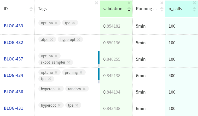
I ran 6 experiments:
- Random search (from hyperopt) as a reference
- Tree of Parzen Estimator search strategies for both Optuna and Hyperopt
- Adaptive TPE from Hyperopt
- TPE from Optuna with a pruning callback for more runs but within the same time frame. It turns out that 400 runs with pruning takes as much time as 100 runs without it.
- Optuna with Random Forest surrogate model from skopt.Sampler
You may want to scroll down to the Example Script at the end.
If you want to explore all of those experiments in more detail you can simply go to the experiment dashboard.
Note:
Register for the free tool for experiment tracking and management
Both Optuna and Hyperopt improved over the random search which is good.
TPE implementation from Optuna was slightly better than Hyperopt’s Adaptive TPE but not by much. On the other hand, when running hyperparameter optimization, those small improvements are exactly what you are going for.
What is interesting is that TPE implementation from HPO and Optuna give vastly different results on this problem. Maybe the cutoff point between good and bad parameter configurations λ is chosen differently or sampling methods have defaults that work better for this particular problem.
Moreover, using pruning decreased training time by 4x. I could run 400 searches in the time that runs 100 without pruning. On the flip side, using pruning got a lower score. It may be different for your problem but it is important to consider that when making a decision whether to use pruning or not.
For this section, I assigned points based on the improvements over the random search strategy.
- Hyperopt got (0.850 – 0.844)100 = **6*
- Optuna got (0.854 – 0.844)100 = **10*
Experimental results
Optuna = Hyperopt
Jump back to the evaluation criteria ->
Conclusions
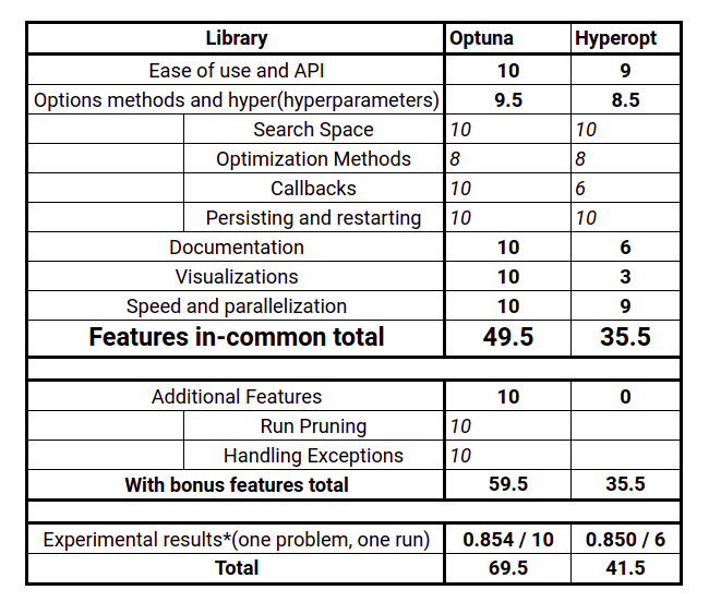
Let’s take a look at the overall scores:
Even if you look at it generously and consider only the features that both libraries share, Optuna is a better framework.
It is on-par or slightly better on all criteria and:
- it has better documentation
- it has way better visualization suite
- it has some features like pruning, callbacks, and exception handling that hyperopt doesn’t support
After doing all this research I am convinced that Optuna is a great library for hyperparameter optimization.
Moreover, I think that you should strongly consider switching from Hyperopt if you were using that in the past.
Example script
import lightgbm as lgb
import neptune
import neptunecontrib.monitoring.optuna as opt_utils
import optuna
import pandas as pd
from sklearn.model_selection import train_test_split

N_ROWS = 10000
TRAIN_PATH = '../data/train.csv'
NUM_BOOST_ROUND = 300
EARLY_STOPPING_ROUNDS = 30
STATIC_PARAMS = {'boosting': 'gbdt',
                 'objective': 'binary',
                 'metric': 'auc',
                 }
N_TRIALS = 100
data = pd.read_csv(TRAIN_PATH, nrows=N_ROWS)

X = data.drop(['ID_code', 'target'], axis=1)
y = data['target']


def train_evaluate(X, y, params):
    X_train, X_valid, y_train, y_valid = train_test_split(X, y, test_size=0.2, random_state=1234)

    train_data = lgb.Dataset(X_train, label=y_train)
    valid_data = lgb.Dataset(X_valid, label=y_valid, reference=train_data)

    model = lgb.train(params, train_data,
                      num_boost_round=NUM_BOOST_ROUND,
                      early_stopping_rounds=EARLY_STOPPING_ROUNDS,
                      valid_sets=[valid_data],
                      valid_names=['valid'])
    score = model.best_score['valid']['auc']
    return score


def objective(trial):
    params = {'learning_rate': trial.suggest_loguniform('learning_rate', 0.01, 0.5),
              'max_depth': trial.suggest_int('max_depth', 1, 30),
              'num_leaves': trial.suggest_int('num_leaves', 2, 100),
              'min_data_in_leaf': trial.suggest_int('min_data_in_leaf', 10, 1000),
              'feature_fraction': trial.suggest_uniform('feature_fraction', 0.1, 1.0),
              'subsample': trial.suggest_uniform('subsample', 0.1, 1.0)}
    all_params = {**params, **STATIC_PARAMS}

    return train_evaluate(X, y, all_params)


neptune.init('jakub-czakon/blog-hpo')
neptune.create_experiment(name='optuna sweep')

monitor = opt_utils.NeptuneMonitor()
study = optuna.create_study(direction='maximize')
study.optimize(objective, n_trials=N_TRIALS, callbacks=[monitor])
opt_utils.log_study(study)

neptune.stop()





Top comments (3)
Nice article.Thanks.
Thanks.
I really wanted it to be useful.
Any comments on how I could have made it even better for your taste?
It’s perfect sir. Thanks.