
AutoAI Overview
AutoAI in Cloud Pak for Data automates ETL(Extract, Transform, and Load) and feature engineering process for relational data, saves data scientists months of manual data prep time and acheives results comparable to top performing data scientists.
The AutoAI graphical tool in Watson Studio automatically analyzes your data and generates candidate model pipelines customized for your predictive modeling problem. These model pipelines are created iteratively as AutoAI analyzes your dataset and discovers data transformations, algorithms, and parameter settings that work best for your problem setting. Results are displayed on a leaderboard, showing the automatically generated model pipelines ranked according to your problem optimization objective.
Collect your input data in a CSV file or files. Where possible, AutoAI will transform the data and impute missing values.
Notes:
- Your data source must contain a minimum of 100 records (rows).
- You can use the IBM Watson Studio Data Refinery tool to prepare and shape your data.
- Data can be a file added as connected data from a networked file system (NFS). Follow the instructions for adding a data connection of the type Mounted Volume. Choose the CSV file to add to the project so you can select it for training data.
AutoAI Process
Using AutoAI, you can build and deploy a machine learning model with sophisticated training features and no coding. The tool does most of the work for you.
AutoAI automatically runs the following tasks to build and evaluate candidate model pipelines:
- Data pre-processing
- Automated model selection
- Automated feature engineering
- Hyperparameter optimization
In this Think Lab, you will see how to join several data sources and then build an AutoAI experiment from the joined data. The scenario we’ll explore in Part A of the Lab is for an outdoor company that wants to project sales for each product in multiple retails stores. You will learn how to join several data sources related to a fictional outdoor store named Go, then build an experiment that uses the data to train a machine learning experiment. You will then deploy the resulting model and use it to predict daily sales for each product Go sells.
Project Requirements
IBM Cloud (Free) Lite Tier Account
Project Setup Steps
- Create an IBM Cloud Lite Tier Account
- Create a Watson Studio Instance
- Provision Watson Machine Learning & Cloud Object Storage Instances
- Create a New Project
- Download the Go Sample Dataset from the Gallery
- Unzip the Go Sample Dataset's .zip File
- Add the Go Sample Datasets to the Project
Project Setup
1. Create an IBM Cloud Lite Tier Account
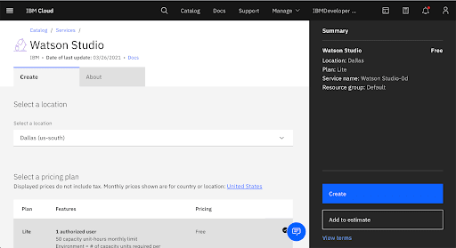
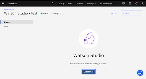
2. Create a Watson Studio Instance

3. Provision Watson Machine Learning & Cloud Object Storage Instances

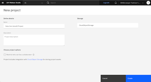
4. Create a New Project

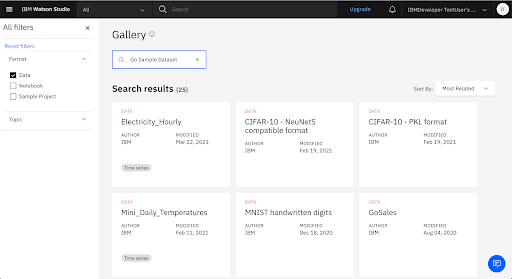
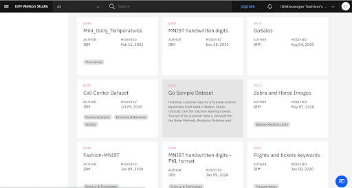
5. Download the Go Sample Dataset from the Gallery


6. Unzip the Go Sample Dataset's .zip File
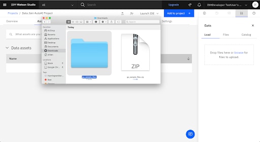
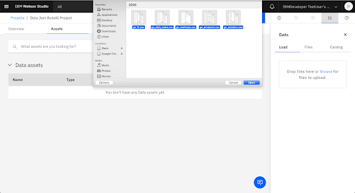
7. Add the Go Sample Datasets to the Project
In Tutorial A of this Think Lab, you will learn how to join several data sources related to a fictional outdoor store named Go, then build an experiment that uses the data to train a machine learning experiment. You will then deploy the resulting model and use it to predict daily sales for each product Go sells.
Joining data also allows for a specialized set of feature transformations and advanced data aggregators. After building the pipelines, you can explore the factors that produced each pipeline.
About the Data

The data you will join contains the following information:
- Daily_sale: the GO company has many retailers selling its outdoor products, the daily sale table is a timeseries of sale records where the DATE and QUANTITY column indicate the sale quantity and the sale date for each product in a retail store.
- Products: this table keeps product information such as product type and product names.
- Retailers: this table keeps retailer infor mation such as retailer names and address.
- Methods: this table keeps order methods such as Via Telephone, Online or Email
- Go: the GO company is interested using this data to predict its daily sale for every product in its retail stores. The prediction target column is QUANTITY in the go table and DATE column indicates the cutoff time when prediction should be made.
Steps Overview
This tutorial presents the basic steps for joining data sets then training a machine learning model using AutoAI:
- Add and join the data
- Train the experiment
- Deploy the trained model
- Test the deployed model
Think Lab - Tutorial A Steps
- Create a New AutoAI Experiment
- Build the Data Join Schema
- Update the AutoAI Experiment Settings
- Run the AutoAI Experiment
- Explore the Holdout & Training Data Insights
- Deploy the Trained Model
- Score the Model
- View the Prediction Results
Think Lab - Tutorial A: Build & Deploy a Data Join Experiment
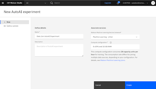
1. Create a New AutoAI Experiment
Add a New AutoAI Experiment to the Project


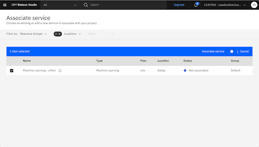
Associate a Machine Learning Service Instance


Select the Go Sample Datasets
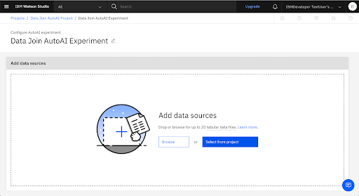

2. Build the Data Join Schema
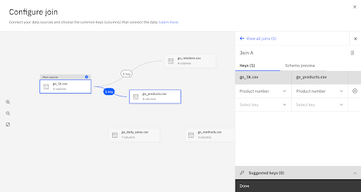
The main source contains the prediction target for the experiment. Select go_1k.csv as the main source, then click Configure join.

In the data join canvas you will create a left join that connects all of the data sources to the main source.
Use the Data Join Table to Build the Schema

Drag from the node on one end of the go_1k.csv box to the node on the end of go_products.csv.
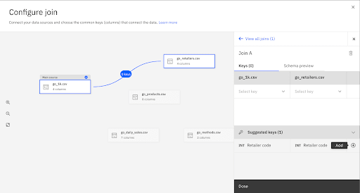
In the panel for configuring the join, click (+) to add the suggested key product_number as the join key.
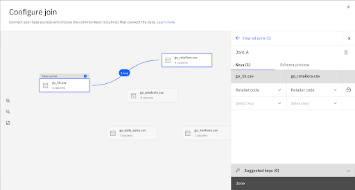
Repeat the data join process until you have joined all the data tables.
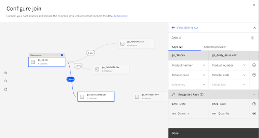

The Completed Data Join Schema Should Look Like This:
Choose Quantity as the column to predict.
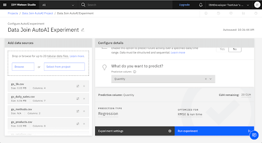
AutoAI analyzes your data and determines that the Quanity column contains a wide range of numeric information, making this data suitable for a regression model. The default metric for a regression model is Root Mean Squared Error (RMSE).
Note:
- Based on analyzing a subset of the data set, AutoAI chooses a default model type: binary classification, multiclass classification, or regression. Binary is selected if the target column has two possible values, multiclass if it has a discrete set of 3 or more values, and regression if the target column is a continuous numeric variable. You can override this selection.
- AutoAI chooses a default metric for optimizing. For example, the default metric for a binary classification model is Accuracy.
- By default, ten percent of the training data is held out to test the performance of the model.
3. Update the AutoAI Experiment Settings
Click Experiment settings

Click the Join Tab on the Data sources Page

Enable the Timestamp Threshold
In the main data table, go_1k.csv, choose Date as the Cutoff time column and enter dd/MM/yyyy as the date format. No data after the date in the cutoff column will be considered for training the pipelines. Note: the data format must exactly match the data or an error results.

In the data table go_daily_sales.csv, choose Date as a timestamp column so that AutoAI can enhance the set of features with timeseries related features. Enter dd/MM/yyyy as the date format. Note: The data format must exactly match the format in the data source or you will get an error running the experiment.
Specify the Runtime Settings
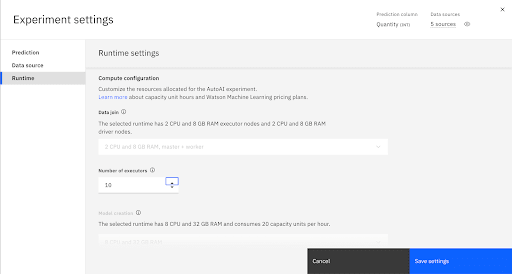
After defining the experiment, you can allocate the resources for training the pipelines. Click Runtime to switch to the Runtime tab. Increase the number of executors to 10. Click Save settings to save the configuration changes.
4. Run the AutoAI Experiment


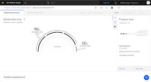
5. Explore the Holdout & Training Data Insights


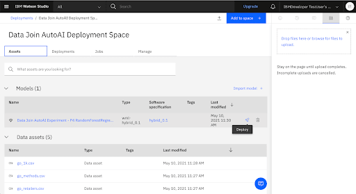
6. Deploy the Trained Model
Click Save as and Select Model

Click Create

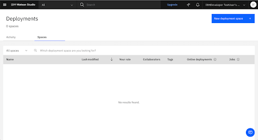
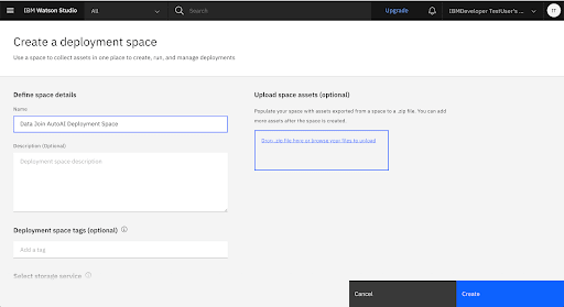
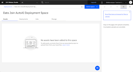
Create a New Deployment Space
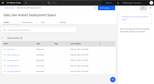
Add the Go Sample Datasets to the Deployment Space

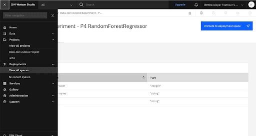
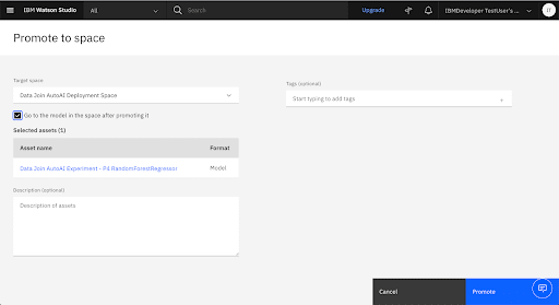
Promote the Trained Model to the Deployment Space

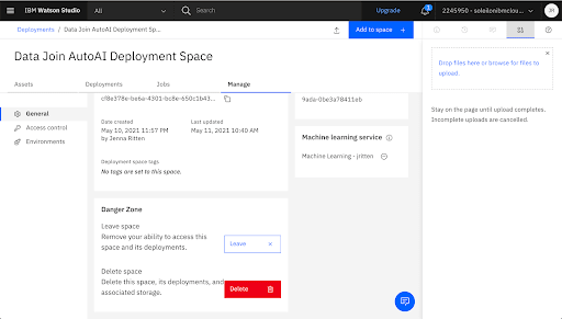
Associate a Machine Learning Service Instance w the Deployment Space


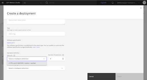
Deploy the Trained Model
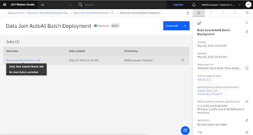
Create a New Batch Deployment

7. Score the Model
To score the model, you create a batch job that will pass new data to the model for processing, then output the predictions to a file. Note: For this tutorial, you will submit the training files as the scoring files as a way to demonstrate the process and view results.
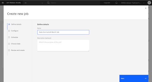
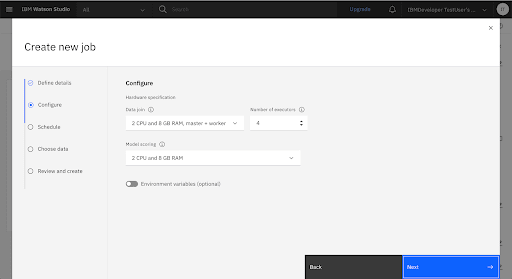
Create a New Batch Job

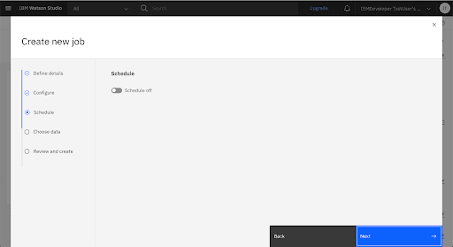
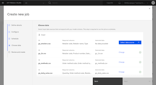
Add the Scoring Files
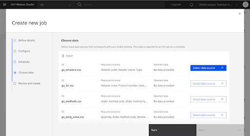
You will see the training files listed. For each training file, click the Edit icon and choose the corresponding scoring file.

WARNING : Schema mismatch. The column types in this data asset do not match the column types in the Model Schema. Click Continue to select anyway.
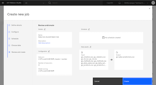
Add go-sales-predictions.csv as the Ouput file name.

Run the Batch Job
When the uploads are complete, click Create to run the job.
View the Batch Job
Wait for the Batch Job to Complete
Starting...

Running...
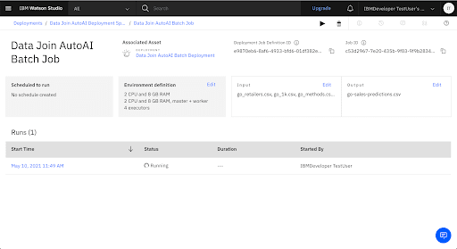
Completed

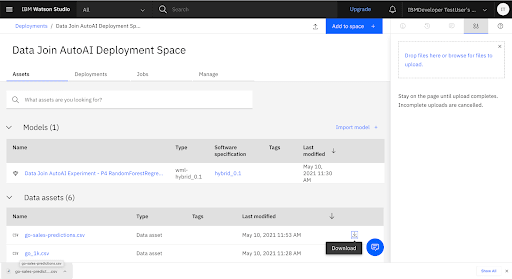
8. View the Prediction Results
Download go-sales-predictions.csv to view the prediction results.
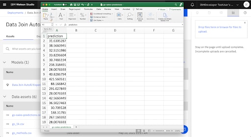
View the go-sales-predictions.csv prediction results in Excel.
Tune in Next Week for Tutorial B: AutoAI Data Join Multi-Classification
In Tutorial B of this Think Lab, you will use IBM AutoAI to automate data analysis for a dataset collected from a fictional call center. The objective of the analysis is to gain more insight into factors that impact customer experience so that the company can improve customer service. The data consists of historical information about customer interaction with call agents, call type, customer wireless plans, and call type resolution.


Top comments (0)