In the previous post, we have learned that how to create a search box with the VLOOKUP function? Similarly, here we are going to discuss the simple way to lookup two tables in Excel by using the VLOOKUP function. Let’s jump into this article!! Get an official version of ** MS Excel** from the following link: https://www.microsoft.com/en-in/microsoft-365/excel
Steps to get the lookup two tables with VLOOKUP:
Now we are going to look up two tables with the VLOOKUP function in Excel by using the search box. Refer to the below example.
- First, we will enter the input values as shown below here we need to find the region of the given state.

- Then, we will select cell E4 , where we need to display the result.
- Click the “Formula” tab from the Ribbon.

- Here, we will select the “Insert Function” option.

- Search for “VLOOKUP” then select to “Go” option.

- The VLOOKUP function will appear in the below box and click on the “OK” button.

- Now, it will open the “Function Arguments” window. In the 1st box , you need to enter the lookup value which you want to be found.
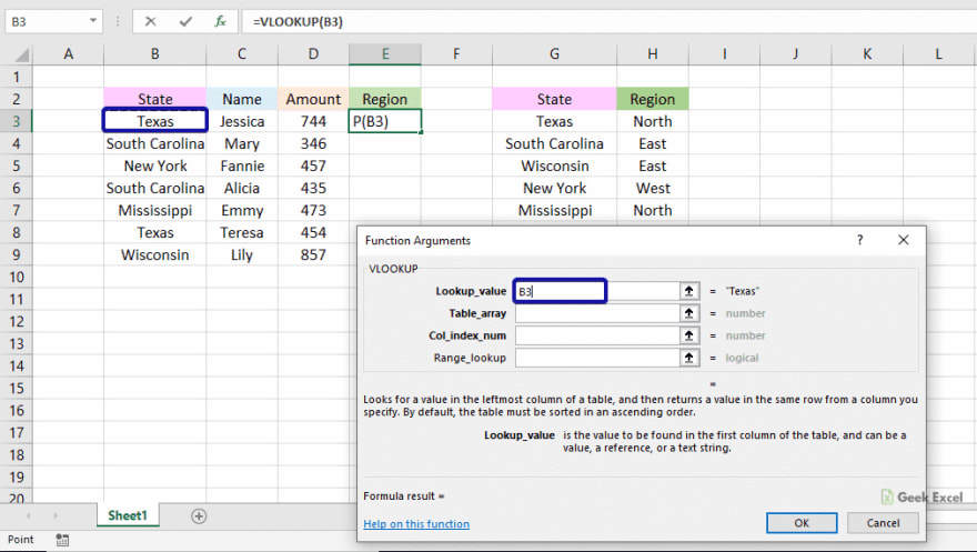
- In the 2nd box, we will select the data range from the worksheet.

- The next box consists of column numbers , where the lookup value will available.

- In the last box, type “False” to search the exact matching value [True= Approximate match], and click the “Ok” button.

- Finally, drag-down the result cell, it will display the results in all cells with a matching value.

Closure:
From this chapter, you have clearly understood the simple steps used to find the lookup value from two tables in Excel based on the VLOOKUP function. If you have any doubt regarding this article or have any other questions related to Excel, let me know in the comments section below. Thank you for Visiting Geek Excel!!

Top comments (0)